Return residuals of a DHARMa simulation
Usage
# S3 method for class 'DHARMa'
residuals(object, quantileFunction = NULL,
  outlierValues = NULL, ...)
Arguments
- object
an object with simulated residuals created by simulateResiduals.
- quantileFunction
optional - a quantile function to transform the uniform 0/1 scaling of DHARMa to another distribution.
- outlierValues
if a quantile function with infinite support (such as qnorm) is used, residuals that are 0/1 are mapped to -Inf / Inf. outlierValues allows to convert -Inf / Inf values to an optional min / max value.
- ...
optional arguments for compatibility with the generic function, no function implemented.
Details
The function accesses the slot $scaledResiduals in a fitted DHARMa object, and optionally transforms the standard DHARMa quantile residuals (which have a uniform distribution) to a particular pdf.
Note
Some of the papers on simulated quantile residuals transforming the residuals (which are natively uniform) back to a normal distribution. I presume this is because of the larger familiarity of most users with normal residuals. Personally, I never considered this desirable, for the reasons explained in https://github.com/florianhartig/DHARMa/issues/39, but with this function, I wanted to give users the option to plot normal residuals if they so wish.
Examples
library(lme4)
testData = createData(sampleSize = 100, overdispersion = 0.5, family = poisson())
fittedModel <- glmer(observedResponse ~ Environment1 + (1|group),
family = "poisson", data = testData)
# simulate residuals (default behavior, conditional on the fitted random effects)
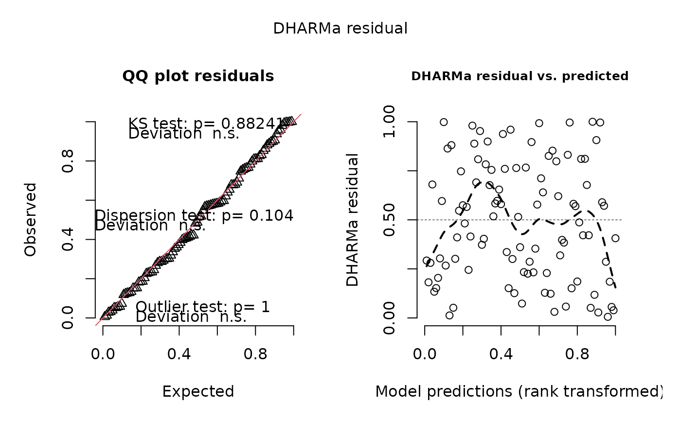
simulationOutput1 <- simulateResiduals(fittedModel = fittedModel)
plot(simulationOutput1, quantreg = FALSE)
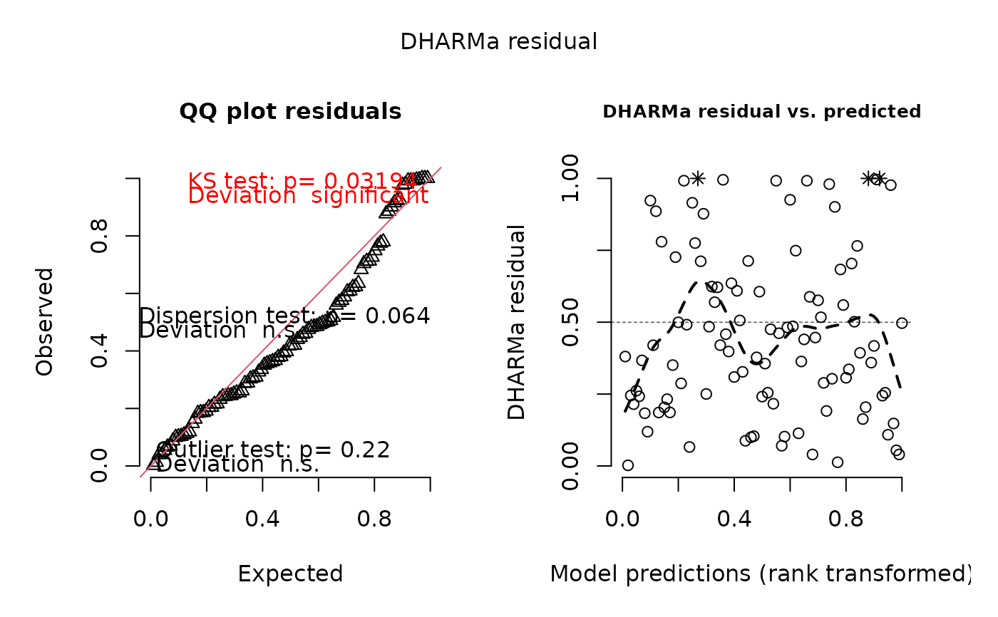
 # simulate residuals unconditional on the fitted random effects (REs are re-simulated)
simulationOutput2 <- simulateResiduals(fittedModel = fittedModel,
simulateREs = "unconditional")
plot(simulationOutput2, quantreg = FALSE)
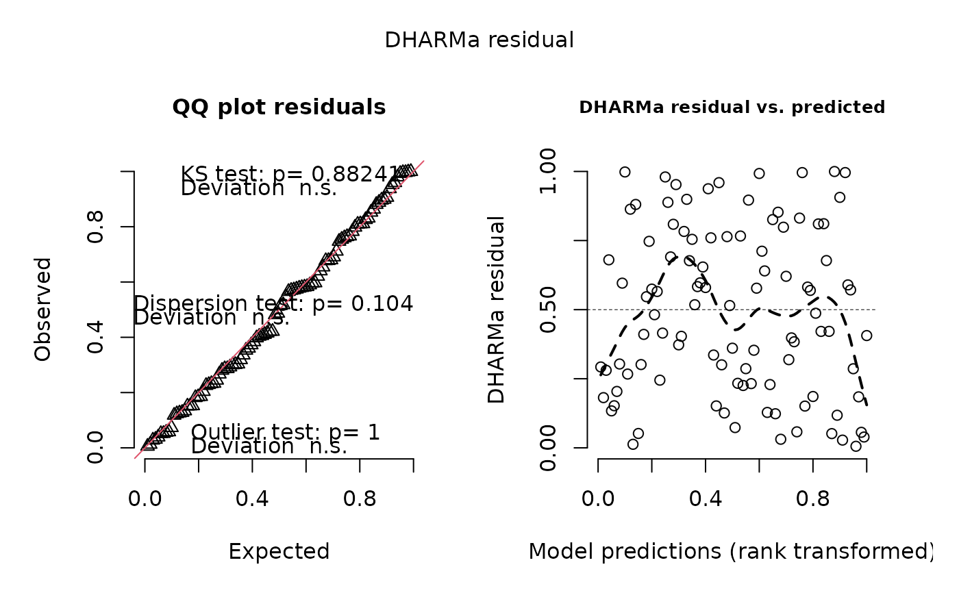
 # simulate residuals user-specified using lme4 syntax (e.g. conditional only on a specific RE)
simulationOutput3 <- simulateResiduals(fittedModel = fittedModel,
simulateREs = "user-specified",
re.form = ~(1|group))
plot(simulationOutput3, quantreg = FALSE)
 # one of the possible test, for other options see ?testResiduals / vignette
testDispersion(simulationOutput1)
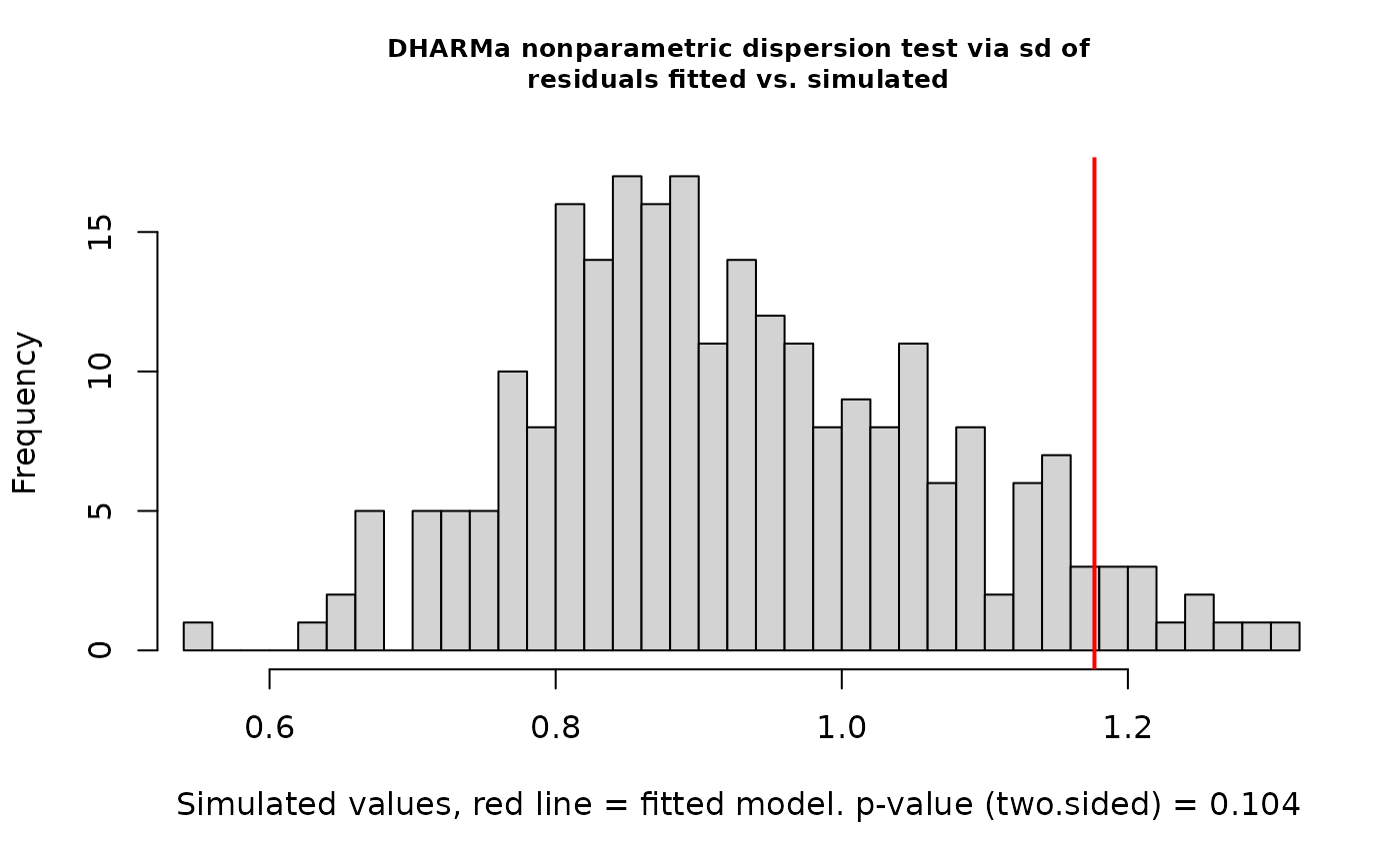 #>
#> DHARMa nonparametric dispersion test via sd of residuals fitted vs.
#> simulated
#>
#> data: simulationOutput
#> dispersion = 1.2711, p-value = 0.104
#> alternative hypothesis: two.sided
#>
# the calculated residuals can be accessed via
residuals(simulationOutput1)
#> [1] 0.620634580 0.266950787 0.998116672 0.952564868 0.810212152 0.225556192
#> [7] 0.117954129 0.577680009 0.133752668 0.185770127 0.640149953 0.073312477
#> [13] 0.992678531 0.152317698 0.581744443 0.747178346 0.810929247 0.031048380
#> [19] 0.204071611 0.244843692 0.403585675 0.303335818 0.228946695 0.863436555
#> [25] 0.151685437 0.995897300 0.569594714 0.051518212 0.880622404 0.514885300
#> [31] 0.360589449 0.301336847 0.012818835 0.937416859 0.232387464 0.782909852
#> [37] 0.852546496 0.487039842 0.280580613 0.383870949 0.580004219 0.397818764
#> [43] 0.896283520 0.481714232 0.056181687 0.546743376 0.825875100 0.353121945
#> [49] 0.421411893 0.754450159 0.051999741 0.759808604 0.711481884 0.184575561
#> [55] 0.798358203 0.808871603 0.766435867 0.300412906 0.574352341 0.126099316
#> [61] 0.039171829 0.286210237 0.677588822 0.596995997 0.571358071 0.151107279
#> [67] 0.831241827 0.583411904 0.959549489 0.410474619 0.690793881 0.286498899
#> [73] 0.123338922 0.999759164 0.028000000 0.565686787 0.057960191 0.996000000
#> [79] 0.005664088 0.517813340 0.128155211 0.415172259 0.372634563 0.899201555
#> [85] 0.292651966 0.595901202 0.764137404 0.906254324 0.589586888 0.680222335
#> [91] 0.654369027 0.181675965 0.233500817 0.318947267 0.677166516 0.406242840
#> [97] 0.980071967 0.888253543 0.335840215 0.421271530
# transform residuals to other pdf, see ?residuals.DHARMa for details
residuals(simulationOutput1, quantileFunction = qnorm, outlierValues = c(-7,7))
#> [1] 0.30714785 -0.62206128 2.89707014 1.67024821 0.87867836 -0.75356181
#> [7] -1.18527621 0.19596191 -1.10882580 -0.89359195 0.35885964 -1.45155653
#> [13] 2.44109164 -1.02654366 0.20635821 0.66563675 0.88132580 -1.86560421
#> [19] -0.82716557 -0.69080613 -0.24407679 -0.51483026 -0.74232014 1.09589006
#> [25] -1.02923156 2.64349905 0.17534243 -1.63030797 1.17810389 0.03732057
#> [31] -0.35688367 -0.52055946 -2.23165658 1.53344487 -0.73100692 0.78205833
#> [37] 1.04741762 -0.03249201 -0.58111756 -0.29532987 0.20190427 -0.25899704
#> [43] 1.26065559 -0.04585169 -1.58765942 0.11743765 0.93798951 -0.37690542
#> [49] -0.19828283 0.68856082 -1.62576582 0.70568702 0.55771907 -0.89806458
#> [55] 0.83577127 0.87374563 0.72715948 -0.52321332 0.18746595 -1.14502541
#> [61] -1.76037847 -0.56449034 0.46096689 0.24557918 0.17983277 -1.03169599
#> [67] 0.95908417 0.21062975 1.74548189 -0.22632425 0.49810188 -0.56364200
#> [73] -1.15845637 3.49074664 -1.91103565 0.16540347 -1.57213010 2.65206981
#> [79] -2.53240900 0.04466627 -1.13515490 -0.21425973 -0.32488366 1.27701518
#> [85] -0.54565380 0.24275190 0.71967489 1.31803673 0.22648243 0.46832061
#> [91] 0.39714309 -0.90899658 -0.72736623 -0.47064463 0.45978999 -0.23722057
#> [97] 2.05523754 1.21729259 -0.42384284 -0.19864166
# get residuals that are outside the simulation envelope
outliers(simulationOutput1)
#> integer(0)
# calculating aggregated residuals per group
# group here specified as formula (recommended)
# but you can also use a variable from your environment, e.g. testData$group
simulationOutput4 = recalculateResiduals(simulationOutput1, group = ~group)
plot(simulationOutput4, quantreg = FALSE)
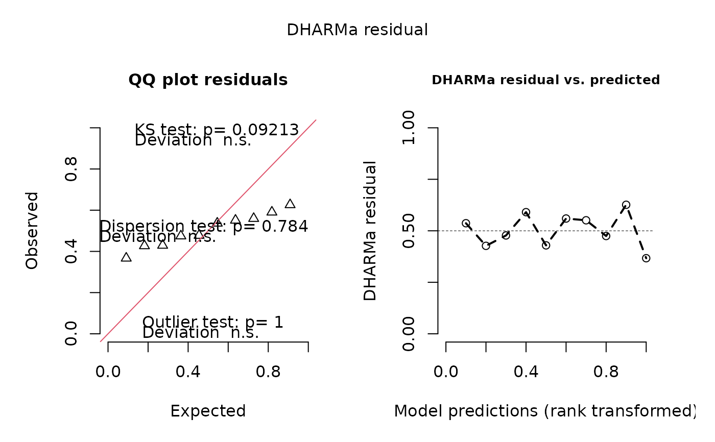 # we see one residual point per RE
# with group as variable in your environment
# but then you need to exclude NAs by hand
simulationOutput5 = recalculateResiduals(simulationOutput1, group = testData$group)
# calculating residuals only for subset of the data
simulationOutput6 = recalculateResiduals(simulationOutput1, sel = testData$group == 1)
plot(simulationOutput6, quantreg = FALSE)
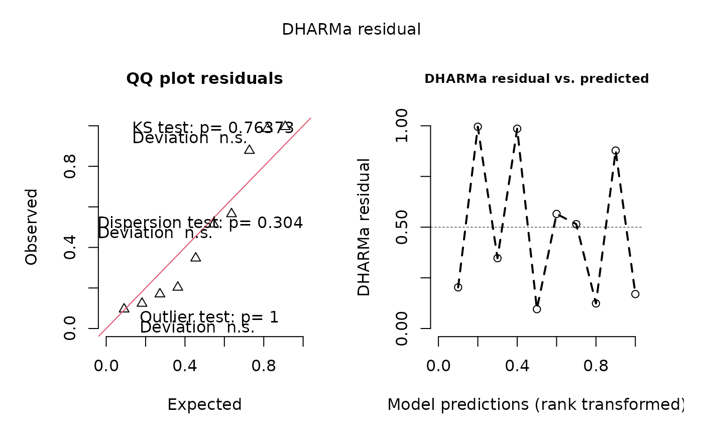 # or with sel as formula
simulationOutput7 = recalculateResiduals(simulationOutput1, sel = ~Environment1<0.5)
# as condition based on a variable in your environment
simulationOutput8 = recalculateResiduals(simulationOutput1, sel = testData$Environment1<0.5)
# or combine group and sel
simulationOutput9 = recalculateResiduals(simulationOutput1, group = ~group, sel = ~Environment1<0.5)
# or as subset of rows
# (note: order of rows is based on residuals, not on original dataframe)
# so be careful with NAs!
simulationOutput10 = recalculateResiduals(simulationOutput1, sel = 1:20)