Matrix of Hoeffding's D Statistics

Computes a matrix of Hoeffding's (1948) D statistics for all possible pairs of columns of a matrix. D is a measure of the distance between F(x,y) and G(x)H(y), where F(x,y) is the joint CDF of X and Y, and G and H are marginal CDFs. Missing values are deleted in pairs rather than deleting all rows of x having any missing variables. The D statistic is robust against a wide variety of alternatives to independence, such as non-monotonic relationships. The larger the value of D, the more dependent are X and Y (for many types of dependencies). D used here is 30 times Hoeffding's original D, and ranges from -0.5 to 1.0 if there are no ties in the data. print.hoeffd prints the information derived by hoeffd. The higher the value of D, the more dependent are x and y. hoeffd also computes the mean and maximum absolute values of the difference between the joint empirical CDF and the product of the marginal empirical CDFs.

hoeffd(x, y)
# S3 method for class 'hoeffd'
print(x, ...)

Arguments

x

a numeric matrix with at least 5 rows and at least 2 columns (if y is absent), or an object created by hoeffd

y

a numeric vector or matrix which will be concatenated to x

...

ignored

Value

a list with elements D, the matrix of D statistics, n the matrix of number of observations used in analyzing each pair of variables, and P, the asymptotic P-values. Pairs with fewer than 5 non-missing values have the D statistic set to NA. The diagonals of n are the number of non-NAs for the single variable corresponding to that row and column.

Details

Uses midranks in case of ties, as described by Hollander and Wolfe. P-values are approximated by linear interpolation on the table in Hollander and Wolfe, which uses the asymptotically equivalent Blum-Kiefer-Rosenblatt statistic. For P<.0001 or >0.5, P values are computed using a well-fitting linear regression function in log P vs. the test statistic. Ranks (but not bivariate ranks) are computed using efficient algorithms (see reference 3).

Author

Frank Harrell
Department of Biostatistics
Vanderbilt University
fh@fharrell.com

References

Hoeffding W. (1948): A non-parametric test of independence. Ann Math Stat 19:546–57.

Hollander M. and Wolfe D.A. (1973). Nonparametric Statistical Methods, pp. 228–235, 423. New York: Wiley.

Press WH, Flannery BP, Teukolsky SA, Vetterling, WT (1988): Numerical Recipes in C. Cambridge: Cambridge University Press.

See also

rcorr, varclus

Examples

x <- c(-2, -1, 0, 1, 2)
y <- c(4,   1, 0, 1, 4)
z <- c(1,   2, 3, 4, NA)
q <- c(1,   2, 3, 4, 5)
hoeffd(cbind(x,y,z,q))
#> D
#>       x     y     z     q
#> x 1e+00 0e+00 3e+50 1e+00
#> y 0e+00 1e+00 3e+50 0e+00
#> z 3e+50 3e+50 1e+00 3e+50
#> q 1e+00 0e+00 3e+50 1e+00
#> 
#> avg|F(x,y)-G(x)H(y)|
#>      x    y z    q
#> x 0.00 0.04 0 0.16
#> y 0.04 0.00 0 0.04
#> z 0.00 0.00 0 0.00
#> q 0.16 0.04 0 0.00
#> 
#> max|F(x,y)-G(x)H(y)|
#>      x   y z    q
#> x 0.00 0.1 0 0.24
#> y 0.10 0.0 0 0.10
#> z 0.00 0.0 0 0.00
#> q 0.24 0.1 0 0.00
#> 
#> n
#>   x y z q
#> x 5 5 4 5
#> y 5 5 4 5
#> z 4 4 4 4
#> q 5 5 4 5
#> 
#> P
#>   x     y     z     q    
#> x       0.363 0.000 0.000
#> y 0.363       0.000 0.363
#> z 0.000 0.000       0.000
#> q 0.000 0.363 0.000      


# Hoeffding's test can detect even one-to-many dependency
set.seed(1)
x <- seq(-10,10,length=200)
y <- x*sign(runif(200,-1,1))
plot(x,y)

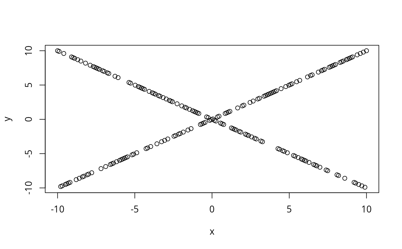hoeffd(x,y)
#> D
#>      x    y
#> x 1.00 0.06
#> y 0.06 1.00
#> 
#> avg|F(x,y)-G(x)H(y)|
#>        x      y
#> x 0.0000 0.0407
#> y 0.0407 0.0000
#> 
#> max|F(x,y)-G(x)H(y)|
#>        x      y
#> x 0.0000 0.0763
#> y 0.0763 0.0000
#> 
#> n= 200 
#> 
#> P
#>   x  y 
#> x     0
#> y  0