Ridge Regression

Fit a linear model by ridge regression.

lm.ridge(formula, data, subset, na.action, lambda = 0, model = FALSE,
         x = FALSE, y = FALSE, contrasts = NULL, ...)
select(obj)

Arguments

formula

a formula expression as for regression models, of the form response ~ predictors. See the documentation of formula for other details. offset terms are allowed.

data

an optional data frame, list or environment in which to interpret the variables occurring in formula.

subset

expression saying which subset of the rows of the data should be used in the fit. All observations are included by default.

na.action

a function to filter missing data.

lambda

A scalar or vector of ridge constants.

model

should the model frame be returned? Not implemented.

x

should the design matrix be returned? Not implemented.

y

should the response be returned? Not implemented.

contrasts

a list of contrasts to be used for some or all of factor terms in the formula. See the contrasts.arg of model.matrix.default.

...

additional arguments to lm.fit.

obj

an R object, such as an "lm.ridge" fit.

Details

If an intercept is present in the model, its coefficient is not penalized. (If you want to penalize an intercept, put in your own constant term and remove the intercept.)

Value

A list with components

coef

matrix of coefficients, one row for each value of lambda. Note that these are not on the original scale and are for use by the coef method.

scales

scalings used on the X matrix.

Inter

was intercept included?

lambda

vector of lambda values

ym

mean of y

xm

column means of x matrix

GCV

vector of GCV values

kHKB

HKB estimate of the ridge constant.

kLW

L-W estimate of the ridge constant.

References

Brown, P. J. (1994) Measurement, Regression and Calibration Oxford.

See also

lm

Examples

longley # not the same as the S-PLUS dataset
#>      GNP.deflator     GNP Unemployed Armed.Forces Population Year Employed
#> 1947         83.0 234.289      235.6        159.0    107.608 1947   60.323
#> 1948         88.5 259.426      232.5        145.6    108.632 1948   61.122
#> 1949         88.2 258.054      368.2        161.6    109.773 1949   60.171
#> 1950         89.5 284.599      335.1        165.0    110.929 1950   61.187
#> 1951         96.2 328.975      209.9        309.9    112.075 1951   63.221
#> 1952         98.1 346.999      193.2        359.4    113.270 1952   63.639
#> 1953         99.0 365.385      187.0        354.7    115.094 1953   64.989
#> 1954        100.0 363.112      357.8        335.0    116.219 1954   63.761
#> 1955        101.2 397.469      290.4        304.8    117.388 1955   66.019
#> 1956        104.6 419.180      282.2        285.7    118.734 1956   67.857
#> 1957        108.4 442.769      293.6        279.8    120.445 1957   68.169
#> 1958        110.8 444.546      468.1        263.7    121.950 1958   66.513
#> 1959        112.6 482.704      381.3        255.2    123.366 1959   68.655
#> 1960        114.2 502.601      393.1        251.4    125.368 1960   69.564
#> 1961        115.7 518.173      480.6        257.2    127.852 1961   69.331
#> 1962        116.9 554.894      400.7        282.7    130.081 1962   70.551
names(longley)[1] <- "y"
lm.ridge(y ~ ., longley)
#>                         GNP    Unemployed  Armed.Forces    Population 
#> 2946.85636017    0.26352725    0.03648291    0.01116105   -1.73702984 
#>          Year      Employed 
#>   -1.41879853    0.23128785 
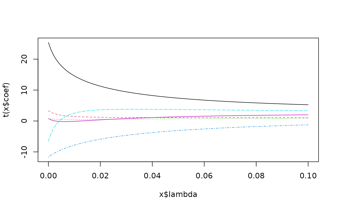
plot(lm.ridge(y ~ ., longley,
              lambda = seq(0,0.1,0.001)))

select(lm.ridge(y ~ ., longley,
               lambda = seq(0,0.1,0.0001)))
#> modified HKB estimator is 0.006836982 
#> modified L-W estimator is 0.05267247 
#> smallest value of GCV  at 0.0057