House Insulation: Whiteside's Data

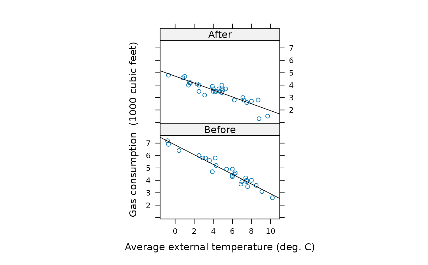
Mr Derek Whiteside of the UK Building Research Station recorded the weekly gas consumption and average external temperature at his own house in south-east England for two heating seasons, one of 26 weeks before, and one of 30 weeks after cavity-wall insulation was installed. The object of the exercise was to assess the effect of the insulation on gas consumption.

whiteside

Format

The whiteside data frame has 56 rows and 3 columns.:

Insul

A factor, before or after insulation.

Temp

Purportedly the average outside temperature in degrees Celsius. (These values is far too low for any 56-week period in the 1960s in South-East England. It might be the weekly average of daily minima.)

Gas

The weekly gas consumption in 1000s of cubic feet.

Source

A data set collected in the 1960s by Mr Derek Whiteside of the UK Building Research Station. Reported by

Hand, D. J., Daly, F., McConway, K., Lunn, D. and Ostrowski, E. eds (1993) A Handbook of Small Data Sets. Chapman & Hall, p. 69.

References

Venables, W. N. and Ripley, B. D. (2002) Modern Applied Statistics with S. Fourth edition. Springer.

Examples

require(lattice)
#> Loading required package: lattice
xyplot(Gas ~ Temp | Insul, whiteside, panel =
  function(x, y, ...) {
    panel.xyplot(x, y, ...)
    panel.lmline(x, y, ...)
  }, xlab = "Average external temperature (deg. C)",
  ylab = "Gas consumption  (1000 cubic feet)", aspect = "xy",
  strip = function(...) strip.default(..., style = 1))


gasB <- lm(Gas ~ Temp, whiteside, subset = Insul=="Before")
gasA <- update(gasB, subset = Insul=="After")
summary(gasB)
#> 
#> Call:
#> lm(formula = Gas ~ Temp, data = whiteside, subset = Insul == 
#>     "Before")
#> 
#> Residuals:
#>     Min      1Q  Median      3Q     Max 
#> -0.6202 -0.1995  0.0607  0.1677  0.5978 
#> 
#> Coefficients:
#>             Estimate Std. Error t value Pr(>|t|)    
#> (Intercept)   6.8538     0.1184    57.9   <2e-16 ***
#> Temp         -0.3932     0.0196   -20.1   <2e-16 ***
#> ---
#> Signif. codes:  0 ‘***’ 0.001 ‘**’ 0.01 ‘*’ 0.05 ‘.’ 0.1 ‘ ’ 1
#> 
#> Residual standard error: 0.281 on 24 degrees of freedom
#> Multiple R-squared:  0.944,	Adjusted R-squared:  0.941 
#> F-statistic:  403 on 1 and 24 DF,  p-value: <2e-16
#> 
summary(gasA)
#> 
#> Call:
#> lm(formula = Gas ~ Temp, data = whiteside, subset = Insul == 
#>     "After")
#> 
#> Residuals:
#>     Min      1Q  Median      3Q     Max 
#> -0.9780 -0.1108  0.0267  0.2529  0.6380 
#> 
#> Coefficients:
#>             Estimate Std. Error t value Pr(>|t|)    
#> (Intercept)   4.7238     0.1297    36.4   <2e-16 ***
#> Temp         -0.2779     0.0252   -11.0    1e-11 ***
#> ---
#> Signif. codes:  0 ‘***’ 0.001 ‘**’ 0.01 ‘*’ 0.05 ‘.’ 0.1 ‘ ’ 1
#> 
#> Residual standard error: 0.355 on 28 degrees of freedom
#> Multiple R-squared:  0.813,	Adjusted R-squared:  0.806 
#> F-statistic:  122 on 1 and 28 DF,  p-value: 1.05e-11
#> 
gasBA <- lm(Gas ~ Insul/Temp - 1, whiteside)
summary(gasBA)
#> 
#> Call:
#> lm(formula = Gas ~ Insul/Temp - 1, data = whiteside)
#> 
#> Residuals:
#>     Min      1Q  Median      3Q     Max 
#> -0.9780 -0.1801  0.0376  0.2093  0.6380 
#> 
#> Coefficients:
#>                  Estimate Std. Error t value Pr(>|t|)    
#> InsulBefore        6.8538     0.1360    50.4   <2e-16 ***
#> InsulAfter         4.7238     0.1181    40.0   <2e-16 ***
#> InsulBefore:Temp  -0.3932     0.0225   -17.5   <2e-16 ***
#> InsulAfter:Temp   -0.2779     0.0229   -12.1   <2e-16 ***
#> ---
#> Signif. codes:  0 ‘***’ 0.001 ‘**’ 0.01 ‘*’ 0.05 ‘.’ 0.1 ‘ ’ 1
#> 
#> Residual standard error: 0.323 on 52 degrees of freedom
#> Multiple R-squared:  0.995,	Adjusted R-squared:  0.994 
#> F-statistic: 2.39e+03 on 4 and 52 DF,  p-value: <2e-16
#> 

gasQ <- lm(Gas ~ Insul/(Temp + I(Temp^2)) - 1, whiteside)
coef(summary(gasQ))
#>                         Estimate Std. Error t value   Pr(>|t|)
#> InsulBefore            6.7592152  0.1507868 44.8263 4.8546e-42
#> InsulAfter             4.4963739  0.1606679 27.9855 3.3026e-32
#> InsulBefore:Temp      -0.3176587  0.0629652 -5.0450 6.3623e-06
#> InsulAfter:Temp       -0.1379016  0.0730580 -1.8876 6.4896e-02
#> InsulBefore:I(Temp^2) -0.0084726  0.0066247 -1.2789 2.0683e-01
#> InsulAfter:I(Temp^2)  -0.0149795  0.0074471 -2.0114 4.9684e-02

gasPR <- lm(Gas ~ Insul + Temp, whiteside)
anova(gasPR, gasBA)
#> Analysis of Variance Table
#> 
#> Model 1: Gas ~ Insul + Temp
#> Model 2: Gas ~ Insul/Temp - 1
#>   Res.Df  RSS Df Sum of Sq    F  Pr(>F)    
#> 1     53 6.77                              
#> 2     52 5.43  1      1.34 12.9 0.00073 ***
#> ---
#> Signif. codes:  0 ‘***’ 0.001 ‘**’ 0.01 ‘*’ 0.05 ‘.’ 0.1 ‘ ’ 1
options(contrasts = c("contr.treatment", "contr.poly"))
gasBA1 <- lm(Gas ~ Insul*Temp, whiteside)
coef(summary(gasBA1))
#>                 Estimate Std. Error  t value   Pr(>|t|)
#> (Intercept)      6.85383   0.135964  50.4091 7.9974e-46
#> InsulAfter      -2.12998   0.180092 -11.8272 2.3159e-16
#> Temp            -0.39324   0.022487 -17.4874 1.9760e-23
#> InsulAfter:Temp  0.11530   0.032112   3.5907 7.3069e-04