Plot model coefficients

Produce dot-and-whisker plot of the model(-averaged) coefficients, with confidence intervals

coefplot(
  x, lci, uci,
  labels = NULL, width = 0.15,
  shift = 0, horizontal = TRUE,
  main = NULL, xlab = NULL, ylab = NULL,
  xlim = NULL, ylim = NULL,
  labAsExpr = TRUE, mar.adj = TRUE, lab.line = 0.5, 
  lty = par("lty"), lwd = par("lwd"), pch = 21,
  col = par("col"), bg = par("bg"),
  dotcex = par("cex"), dotcol = col,
  staplelty = lty, staplelwd = lwd, staplecol = col,
  zerolty = "dotted", zerolwd = lwd, zerocol = "gray",
  las = 2, ann = TRUE, axes = TRUE, add = FALSE,
  type = "p",
  ...
)

# S3 method for class 'averaging'
plot(
  x,
  full = TRUE, level = 0.95, intercept = TRUE,
  parm = NULL, labels = NULL, width = 0.1,
  shift = max(0.2, width * 2.1 + 0.05),
  horizontal = TRUE, 
  xlim = NULL, ylim = NULL,
  main = "Model-averaged coefficients",
  xlab = NULL, ylab = NULL, 
  add = FALSE,
  ...
)

Arguments

x

either a (possibly named) vector of coefficients (for coefplot), or an "averaging"=model.avg object.

lci, uci

vectors of lower and upper confidence intervals. Alternatively a two-column matrix with columns containing confidence intervals, in which case uci is ignored.

labels

optional vector of coefficient names. By default, names of x are used for labels.

width

width of the staples (= end of whisker).

shift

the amount of perpendicular shift for the dots and whiskers. Useful when adding to an existing plot.

horizontal

logical indicating if the plots should be horizontal; defaults to TRUE.

main

an overall title for the plot: see title.

xlab, ylab

x- and y-axis annotation. Can be suppressed by ann=FALSE.

xlim, ylim

optional, the x and y limits of the plot.

labAsExpr

logical indicating whether the coefficient names should be transformed to expressions to create prettier labels (see plotmath)

mar.adj

logical indicating whether the (left or lower) margin should be expanded to fit the labels

lab.line

margin line for the labels

lty, lwd, pch, col, bg

default line type, line width, point character, foreground colour for all elements, and background colour for open symbols.

dotcex, dotcol

dots point size expansion and colour.

staplelty, staplelwd, staplecol

staple line type, width, and colour.

zerolty, zerolwd, zerocol

zero-line type, line width, colour. Setting zerolty to NA suppresses the line.

las

the style of labels for coefficient names. See par.

ann

logical indicating if axes should be annotated (by xlab and ylab).

axes

a logical value indicating whether both axes should be drawn on the plot.

add

logical, if true add to current plot.

type

if "n", the plot region is left empty, any other value causes the plot being drawn.

...

additional arguments passed to coefplot or more graphical parameters.

full

a logical value specifying whether the “full” model-averaged coefficients are plotted. If FALSE, the “subset”-averaged coefficients are plotted, and both types if NA. See model.avg.

level

the confidence level required.

intercept

logical indicating if intercept should be included in the plot

parm

a specification of which parameters are to be plotted, either a vector of numbers or a vector of names. If missing, all parameters are considered.

Value

An invisible matrix containing coordinates of points and whiskers, or, a two-element list of such, one for each coefficient type in plot.averaging when full is NA.

Details

Plot model(-averaged) coefficients with confidence intervals.

Author

Kamil Bartoń

Examples

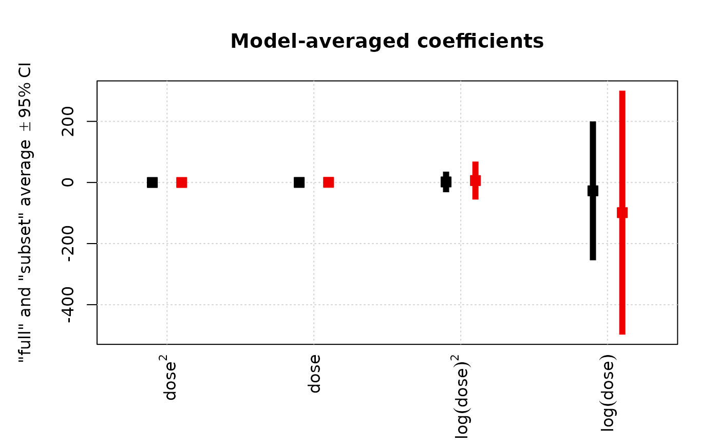
fm <- glm(Prop ~ dose + I(dose^2) + log(dose) + I(log(dose)^2),
  data = Beetle, family = binomial, na.action = na.fail)
ma <- model.avg(dredge(fm))
#> Fixed term is "(Intercept)"

# default coefficient plot:
plot(ma, full = NA, intercept = FALSE)


# Add colours per coefficient type
# Replicate each colour n(=number of coefficients) times
clr <- c("black", "red2")
i <- rep(1:2, each = length(coef(ma)) - 1)
plot(ma, full = NA, intercept = FALSE,
   pch = 22, dotcex = 1.5,
   col = clr[i], bg = clr[i],
   lwd = 6, lend = 1, width = 0, horizontal = 0)


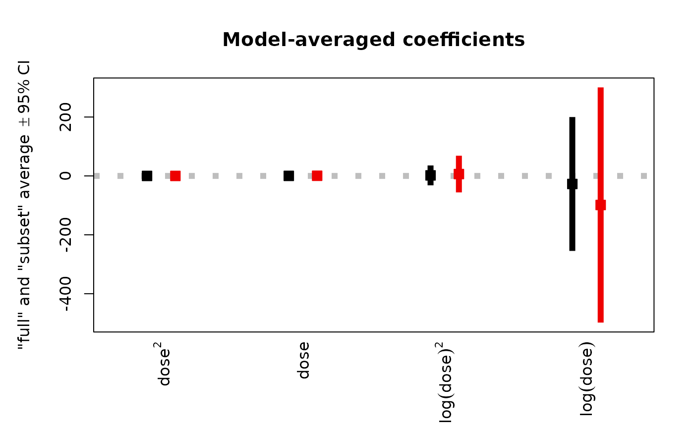# Use `type = "n"` and `add` argument to e.g. add grid beneath the figure
plot(ma, full = NA, intercept = FALSE,
   width = 0, horizontal = FALSE, zerolty = NA, type = "n")
grid()
plot(ma, full = NA, intercept = FALSE,
   pch = 22, dotcex = 1.5,
   col = clr[i], bg = clr[i],
   lwd = 6, lend = 1, width = 0, horizontal = FALSE, add = TRUE)