Visualize model selection table — plot.model.selection • MuMIn

Produces a graphical representation of model weights and terms.

# S3 method for class 'model.selection'
plot(
  x,
  ylab = NULL, xlab = NULL, main = "Model selection table",
  labels = NULL, terms = NULL, labAsExpr = TRUE,
  vlabels = rownames(x), mar.adj = TRUE,
  col = NULL, col.mode = 2,
  bg = "white", border = par("col"),
  par.lab = NULL, par.vlab = NULL,
  axes = TRUE, ann = TRUE,
  ...
)

Arguments

x: a "model.selection" object.
xlab, ylab, main: labels for the x and y axes, and the main title for the plot.
labels: optional, a character vector or an expression containing model term labels (to appear on top side of the plot). Its length must be equal to number of displayed model terms. Defaults to the model term names.
terms: which terms to include (default NULL means all terms).
labAsExpr: logical, indicating whether the term names should be interpreted (parsed) as R expressions for prettier labels. See also plotmath.
vlabels: alternative labels for the table rows (i.e. model names)
mar.adj: logical indicating whether the top and right margin should be enlarged if necessary to fit the labels.
col: vector or a matrix of colours for the non-empty grid cells. See 'Details'. If col is given as a matrix, the colours are applied to rows and columns. How it is done is governed by the argument col.mode.
col.mode: either numeric or "value", specifies cell colouring mode. See 'Details'.
bg: background colour for the empty cells.
border: border colour for cells and axes.
par.lab, par.vlab: optional lists of arguments and graphical parameters for drawing term labels (top axis) and model names (right axis), respectively. Items of par.lab are passed as arguments to mtext, and those of par.vlab are passed to axis.
axes, ann: logical values indicating whether the axis and annotation should appear on the plot.
...: further graphical parameters to be set for the plot.

Details

Colours

If col.mode = 0, the colours are recycled: if col is a matrix, recycling takes place both per row and per column. If col.mode > 0, the colour values in the columns are interpolated and assigned according to the model weights. Higher values shift the colours for models with lower model weights more forward. See also colorRamp. If col.mode < 0 or "value" (partially matched, case-insensitive) and col has two or more elements, colours are used to represent coefficient values: the first element in col is used for categorical predictors, the rest for continuous values. The default is grey for factors and HCL palette "Blue-Red 3" otherwise, ranging from blue for negative values to red for positive ones.

The following arguments are useful for adjusting label size and position in par.lab and par.vlab : cex, las (see par), line and hadj (see mtext and axis).

Author

Kamil Bartoń

Examples

ms <- dredge(lm(formula = y ~ ., data = Cement, na.action = na.fail))
#> Fixed term is "(Intercept)"
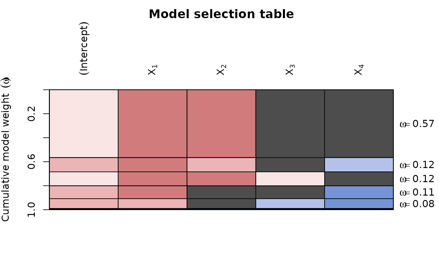
plot(ms,
    # colours by coefficient value:
    col.mode = "value",
    par.lab = list(las = 2, line = 1.2, cex = 1),
    bg = "gray30",
    # change labels for the models to Akaike weights:
    vlabels = parse(text = paste("omega ==", round(Weights(ms), 2)))
    )

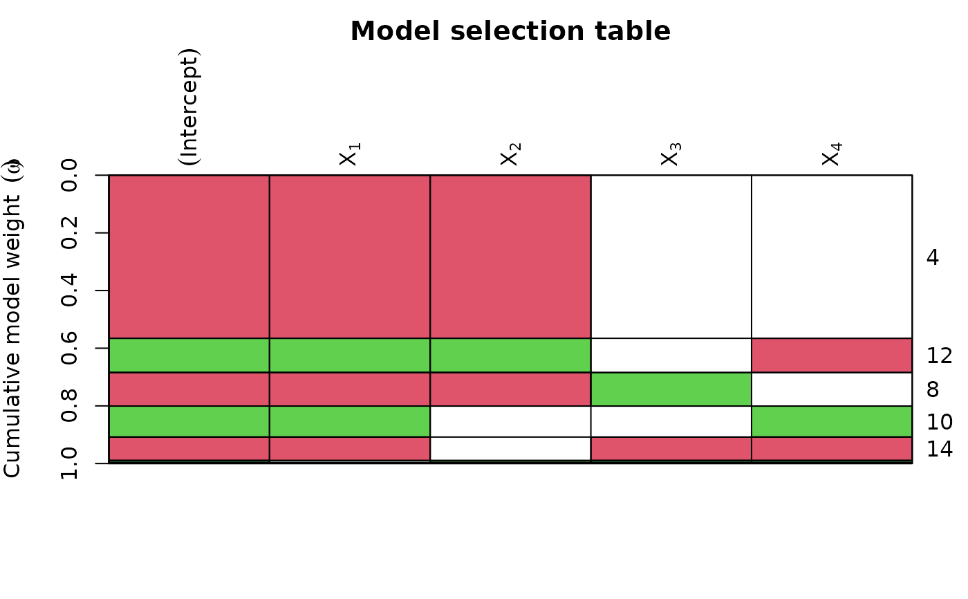
plot(ms, col = 2:3, col.mode = 0) # colour recycled by row

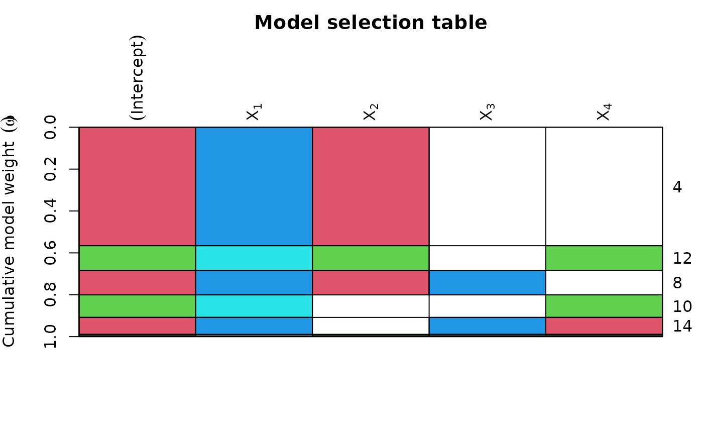
plot(ms, col = cbind(2:3, 4:5), col.mode = 0) # colour recycled by row and column

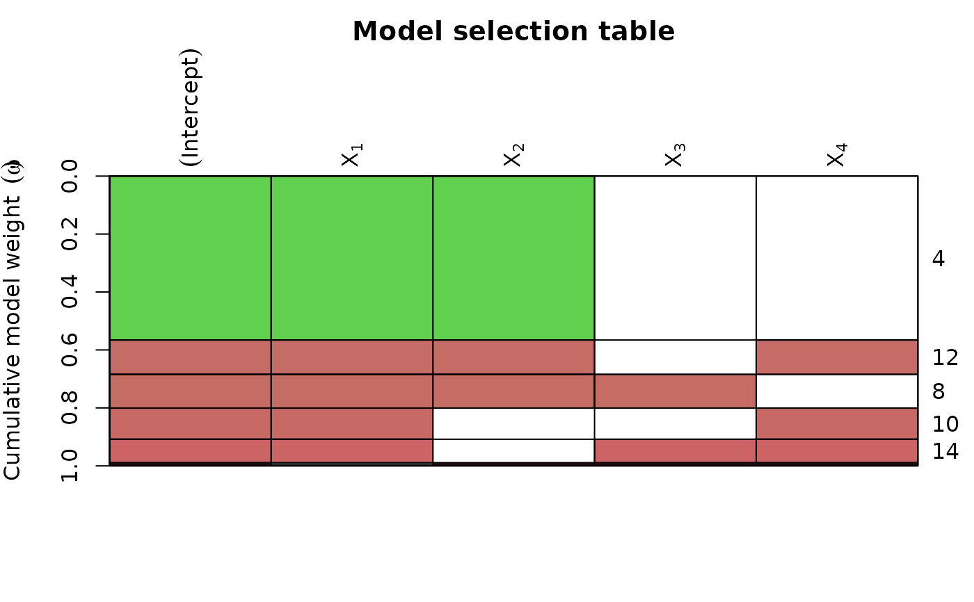
plot(ms, col = 2:3, col.mode = 1) # colour gradient by model weight