Exponential Regression by Asymmetric Maximum Likelihood Estimation

Exponential expectile regression estimated by maximizing an asymmetric likelihood function.

amlexponential(w.aml = 1, parallel = FALSE, imethod = 1, digw = 4,
               link = "loglink")

Arguments

w.aml

Numeric, a vector of positive constants controlling the expectiles. The larger the value the larger the fitted expectile value (the proportion of points below the “w-regression plane”). The default value of unity results in the ordinary maximum likelihood (MLE) solution.

parallel

If w.aml has more than one value then this argument allows the quantile curves to differ by the same amount as a function of the covariates. Setting this to be TRUE should force the quantile curves to not cross (although they may not cross anyway). See CommonVGAMffArguments for more information.

imethod

Integer, either 1 or 2 or 3. Initialization method. Choose another value if convergence fails.

digw

Passed into Round as the digits argument for the w.aml values; used cosmetically for labelling.

link

See exponential and the warning below.

Details

The general methodology behind this VGAM family function is given in Efron (1992) and full details can be obtained there. This model is essentially an exponential regression model (see exponential) but the usual deviance is replaced by an asymmetric squared error loss function; it is multiplied by \(w.aml\) for positive residuals. The solution is the set of regression coefficients that minimize the sum of these deviance-type values over the data set, weighted by the weights argument (so that it can contain frequencies). Newton-Raphson estimation is used here.

Value

An object of class "vglmff" (see vglmff-class). The object is used by modelling functions such as vglm and vgam.

References

Efron, B. (1992). Poisson overdispersion estimates based on the method of asymmetric maximum likelihood. Journal of the American Statistical Association, 87, 98–107.

Author

Thomas W. Yee

Note

On fitting, the extra slot has list components "w.aml" and "percentile". The latter is the percent of observations below the “w-regression plane”, which is the fitted values. Also, the individual deviance values corresponding to each element of the argument w.aml is stored in the extra slot.

For amlexponential objects, methods functions for the generic functions qtplot and cdf have not been written yet.

See amlpoisson about comments on the jargon, e.g., expectiles etc.

In this documentation the word quantile can often be interchangeably replaced by expectile (things are informal here).

Warning

Note that the link argument of exponential and amlexponential are currently different: one is the rate parameter and the other is the mean (expectile) parameter.

If w.aml has more than one value then the value returned by deviance is the sum of all the (weighted) deviances taken over all the w.aml values. See Equation (1.6) of Efron (1992).

Examples

nn <- 2000
mydat <- data.frame(x = seq(0, 1, length = nn))
mydat <- transform(mydat,
                   mu = loglink(-0 + 1.5*x + 0.2*x^2, inverse = TRUE))
mydat <- transform(mydat, mu = loglink(0 - sin(8*x), inverse = TRUE))
mydat <- transform(mydat,  y = rexp(nn, rate = 1/mu))
(fit <- vgam(y ~ s(x, df=5), amlexponential(w=c(0.001, 0.1, 0.5, 5, 60)),
             mydat, trace = TRUE))
#> VGAM  s.vam  loop  1 :  deviance = 15338.5261
#> VGAM  s.vam  loop  2 :  deviance = 11922.2259
#> VGAM  s.vam  loop  3 :  deviance = 11390.7305
#> VGAM  s.vam  loop  4 :  deviance = 11303.912
#> VGAM  s.vam  loop  5 :  deviance = 11254.9563
#> VGAM  s.vam  loop  6 :  deviance = 11234.07
#> VGAM  s.vam  loop  7 :  deviance = 11227.2618
#> VGAM  s.vam  loop  8 :  deviance = 11226.0931
#> VGAM  s.vam  loop  9 :  deviance = 11226.0089
#> VGAM  s.vam  loop  10 :  deviance = 11226.0051
#> VGAM  s.vam  loop  11 :  deviance = 11226.0046
#> VGAM  s.vam  loop  12 :  deviance = 11226.0046
#> 
#> Call:
#> vgam(formula = y ~ s(x, df = 5), family = amlexponential(w = c(0.001, 
#>     0.1, 0.5, 5, 60)), data = mydat, trace = TRUE)
#> 
#> 
#> Degrees of Freedom: 10000 Total; 9969.71 Residual
#> Residual deviance: 11226 
fit@extra
#> $w.aml
#> [1] 1e-03 1e-01 5e-01 5e+00 6e+01
#> 
#> $M
#> [1] 5
#> 
#> $n
#> [1] 2000
#> 
#> $y.names
#> [1] "w.aml = 0.001" "w.aml = 0.1"   "w.aml = 0.5"   "w.aml = 5"    
#> [5] "w.aml = 60"   
#> 
#> $individual
#> [1] TRUE
#> 
#> $percentile
#> w.aml = 0.001   w.aml = 0.1   w.aml = 0.5     w.aml = 5    w.aml = 60 
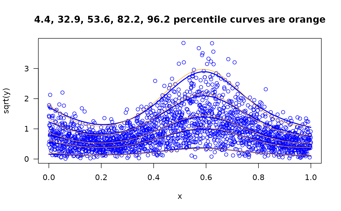
#>          4.40         32.85         53.65         82.15         96.15 
#> 
#> $deviance
#> w.aml = 0.001   w.aml = 0.1   w.aml = 0.5     w.aml = 5    w.aml = 60 
#>      166.7813     1130.4200     1894.9898     3277.2637     4756.5499 
#> 

if (FALSE)  # These plots are against the sqrt scale (to increase clarity)
par(mfrow = c(1,2))
# Quantile plot
with(mydat, plot(x, sqrt(y), col = "blue", las = 1, main =
     paste(paste(round(fit@extra$percentile, digits = 1), collapse=", "),
           "percentile-expectile curves")))
with(mydat, matlines(x, sqrt(fitted(fit)), lwd = 2, col = "blue", lty=1))


# Compare the fitted expectiles with the quantiles
with(mydat, plot(x, sqrt(y), col = "blue", las = 1, main =
     paste(paste(round(fit@extra$percentile, digits = 1), collapse=", "),
           "percentile curves are orange")))
with(mydat, matlines(x, sqrt(fitted(fit)), lwd = 2, col = "blue", lty=1))

for (ii in fit@extra$percentile)
  with(mydat, matlines(x, sqrt(qexp(p = ii/100, rate = 1/mu)),
                       col = "orange"))  # \dontrun{}