The Laplace Distribution

Density, distribution function, quantile function and random generation for the Laplace distribution with location parameter location and scale parameter scale.

dlaplace(x, location = 0, scale = 1, log = FALSE)
plaplace(q, location = 0, scale = 1, lower.tail = TRUE, log.p = FALSE)
qlaplace(p, location = 0, scale = 1, lower.tail = TRUE, log.p = FALSE)
rlaplace(n, location = 0, scale = 1)

Arguments

x, q

vector of quantiles.

p

vector of probabilities.

n

number of observations. Same as in runif.

location

the location parameter \(a\), which is the mean.

scale

the scale parameter \(b\). Must consist of positive values.

log

Logical. If log = TRUE then the logarithm of the density is returned.

lower.tail, log.p

Same meaning as in pnorm or qnorm.

Details

The Laplace distribution is often known as the double-exponential distribution and, for modelling, has heavier tail than the normal distribution. The Laplace density function is $$f(y) = \frac{1}{2b} \exp \left( - \frac{|y-a|}{b} \right) $$ where \(-\infty<y<\infty\), \(-\infty<a<\infty\) and \(b>0\). The mean is \(a\) and the variance is \(2b^2\).

See laplace, the VGAM family function for estimating the two parameters by maximum likelihood estimation, for formulae and details. Apart from n, all the above arguments may be vectors and are recyled to the appropriate length if necessary.

Value

dlaplace gives the density, plaplace gives the distribution function, qlaplace gives the quantile function, and rlaplace generates random deviates.

References

Forbes, C., Evans, M., Hastings, N. and Peacock, B. (2011). Statistical Distributions, Hoboken, NJ, USA: John Wiley and Sons, Fourth edition.

Author

T. W. Yee and Kai Huang

See also

laplace.

Examples

loc <- 1; b <- 2
y <- rlaplace(n = 100, loc = loc, scale = b)
mean(y)  # sample mean
#> [1] 1.376246
loc      # population mean
#> [1] 1
var(y)   # sample variance
#> [1] 7.528536
2 * b^2  # population variance
#> [1] 8

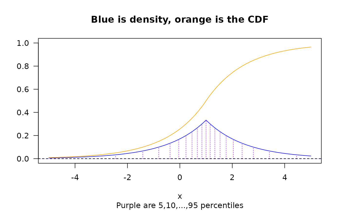
if (FALSE)  loc <- 0; b <- 1.5; x <- seq(-5, 5, by = 0.01)
plot(x, dlaplace(x, loc, b), type = "l", col = "blue",
     main = "Blue is density, orange is the CDF", ylim = c(0,1),
     sub = "Purple are 5,10,...,95 percentiles", las = 1, ylab = "")
abline(h = 0, col = "blue", lty = 2)
lines(qlaplace(seq(0.05,0.95,by = 0.05), loc, b),
      dlaplace(qlaplace(seq(0.05, 0.95, by = 0.05), loc, b), loc, b),
      col = "purple", lty = 3, type = "h")
lines(x, plaplace(x, loc, b), type = "l", col = "orange")
abline(h = 0, lty = 2)  # \dontrun{}


plaplace(qlaplace(seq(0.05, 0.95, by = 0.05), loc, b), loc, b)
#>  [1] 0.05 0.10 0.15 0.20 0.25 0.30 0.35 0.40 0.45 0.50 0.55 0.60 0.65 0.70 0.75
#> [16] 0.80 0.85 0.90 0.95