The Poisson Lognormal Distribution

Density, distribution function and random generation for the Poisson lognormal distribution.

dpolono(x, meanlog = 0, sdlog = 1, bigx = 170, ...)
ppolono(q, meanlog = 0, sdlog = 1,
        isOne = 1 - sqrt( .Machine$double.eps ), ...)
rpolono(n, meanlog = 0, sdlog = 1)

Arguments

x, q

vector of quantiles.

n

number of observations. If length(n) > 1 then the length is taken to be the number required.

meanlog, sdlog

the mean and standard deviation of the normal distribution (on the log scale). They match the arguments in Lognormal.

bigx

Numeric. This argument is for handling large values of x and/or when integrate fails. A first order Taylor series approximation [Equation (7) of Bulmer (1974)] is used at values of x that are greater or equal to this argument. For bigx = 10, he showed that the approximation has a relative error less than 0.001 for values of meanlog and sdlog “likely to be encountered in practice”. The argument can be assigned Inf in which case the approximation is not used.

isOne

Used to test whether the cumulative probabilities have effectively reached unity.

...

Arguments passed into integrate.

Value

dpolono gives the density, ppolono gives the distribution function, and rpolono generates random deviates.

References

Bulmer, M. G. (1974). On fitting the Poisson lognormal distribution to species-abundance data. Biometrics, 30, 101–110.

Author

T. W. Yee. Some anonymous soul kindly wrote ppolono() and improved the original dpolono().

Details

The Poisson lognormal distribution is similar to the negative binomial in that it can be motivated by a Poisson distribution whose mean parameter comes from a right skewed distribution (gamma for the negative binomial and lognormal for the Poisson lognormal distribution).

Note

By default, dpolono involves numerical integration that is performed using integrate. Consequently, computations are very slow and numerical problems may occur (if so then the use of ... may be needed). Alternatively, for extreme values of x, meanlog, sdlog, etc., the use of bigx = Inf avoids the call to integrate, however the answer may be a little inaccurate.

For the maximum likelihood estimation of the 2 parameters a VGAM family function called polono(), say, has not been written yet.

See also

lognormal, poissonff, negbinomial.

Examples

meanlog <- 0.5; sdlog <- 0.5; yy <- 0:19
sum(proby <- dpolono(yy, m = meanlog, sd = sdlog))  # Should be 1
#> [1] 0.9999955
max(abs(cumsum(proby) - ppolono(yy, m = meanlog, sd = sdlog)))  # 0?
#> [1] 2.220446e-16

if (FALSE)  opar = par(no.readonly = TRUE)
par(mfrow = c(2, 2))
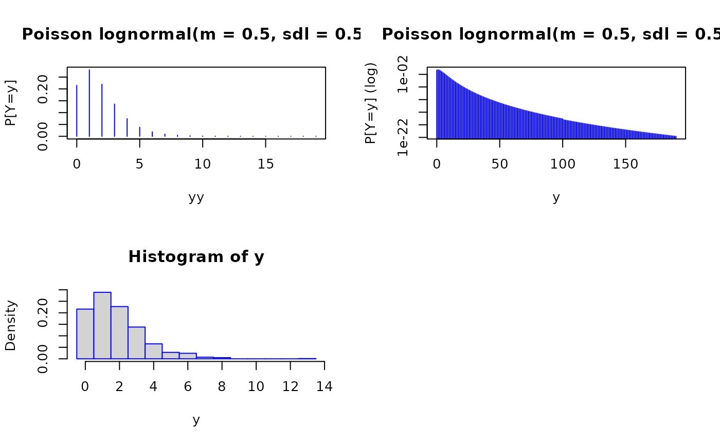
plot(yy, proby, type = "h", col = "blue", ylab = "P[Y=y]", log = "",
     main = paste0("Poisson lognormal(m = ", meanlog,
                  ", sdl = ", sdlog, ")"))

y <- 0:190  # More extreme values; use the approxn & plot on a log scale
(sum(proby <- dpolono(y, m = meanlog, sd = sdlog, bigx = 100)))  # 1?
#> [1] 1
plot(y, proby, type = "h", col = "blue", ylab = "P[Y=y] (log)", log = "y",
     main = paste0("Poisson lognormal(m = ", meanlog,
                  ", sdl = ", sdlog, ")"))  # Note the kink at bigx

# Random number generation
table(y <- rpolono(n = 1000, m = meanlog, sd = sdlog))
#> 
#>   0   1   2   3   4   5   6   7   8  13 
#> 216 289 227 138  65  28  24   7   5   1 
hist(y, breaks = ((-1):max(y))+0.5, prob = TRUE, border = "blue")
par(opar)  # \dontrun{}
#> Error: object 'opar' not found