Rayleigh Regression Family Function

Estimating the parameter of the Rayleigh distribution by maximum likelihood estimation. Right-censoring is allowed.

rayleigh(lscale = "loglink", nrfs = 1/3 + 0.01,
            oim.mean = TRUE, zero = NULL, parallel = FALSE,
            type.fitted = c("mean", "percentiles", "Qlink"),
            percentiles = 50)
cens.rayleigh(lscale = "loglink", oim = TRUE)

Arguments

lscale

Parameter link function applied to the scale parameter \(b\). See Links for more choices. A log link is the default because \(b\) is positive.

nrfs

Numeric, of length one, with value in \([0,1]\). Weighting factor between Newton-Raphson and Fisher scoring. The value 0 means pure Newton-Raphson, while 1 means pure Fisher scoring. The default value uses a mixture of the two algorithms, and retaining positive-definite working weights.

oim.mean

Logical, used only for intercept-only models. TRUE means the mean of the OIM elements are used as working weights. If TRUE then this argument has top priority for working out the working weights. FALSE means use another algorithm.

oim

Logical. For censored data only, TRUE means the Newton-Raphson algorithm, and FALSE means Fisher scoring.

zero, parallel

Details at CommonVGAMffArguments.

type.fitted, percentiles

See CommonVGAMffArguments for information. Using "Qlink" is for quantile-links in VGAMextra.

Details

The Rayleigh distribution, which is used in physics, has a probability density function that can be written $$f(y) = y \exp(-0.5 (y/b)^2)/b^2$$ for \(y > 0\) and \(b > 0\). The mean of \(Y\) is \(b \sqrt{\pi / 2}\) (returned as the fitted values) and its variance is \(b^2 (4-\pi)/2\).

The VGAM family function cens.rayleigh handles right-censored data (the true value is greater than the observed value). To indicate which type of censoring, input extra = list(rightcensored = vec2) where vec2 is a logical vector the same length as the response. If the component of this list is missing then the logical values are taken to be FALSE. The fitted object has this component stored in the extra slot.

The VGAM family function rayleigh handles multiple responses.

Warning

The theory behind the argument oim is not fully complete.

Value

An object of class "vglmff" (see vglmff-class). The object is used by modelling functions such as vglm, rrvglm and vgam.

References

Forbes, C., Evans, M., Hastings, N. and Peacock, B. (2011). Statistical Distributions, Hoboken, NJ, USA: John Wiley and Sons, Fourth edition.

Author

T. W. Yee

Note

The poisson.points family function is more general so that if ostatistic = 1 and dimension = 2 then it coincides with rayleigh. Other related distributions are the Maxwell and Weibull distributions.

See also

Rayleigh, genrayleigh, riceff, maxwell, weibullR, poisson.points, simulate.vlm.

Examples

nn <- 1000; Scale <- exp(2)
rdata <- data.frame(ystar = rrayleigh(nn, scale = Scale))
fit <- vglm(ystar ~ 1, rayleigh, data = rdata, trace = TRUE)
#> Iteration 1: loglikelihood = -2931.7335
#> Iteration 2: loglikelihood = -2931.7322
#> Iteration 3: loglikelihood = -2931.7322
head(fitted(fit))
#>       [,1]
#> 1 9.304225
#> 2 9.304225
#> 3 9.304225
#> 4 9.304225
#> 5 9.304225
#> 6 9.304225
with(rdata, mean(ystar))
#> [1] 9.362191
coef(fit, matrix = TRUE)
#>             loglink(scale)
#> (Intercept)       2.004677
Coef(fit)
#>    scale 
#> 7.423698 

# Censored data
rdata <- transform(rdata, U = runif(nn, 5, 15))
rdata <- transform(rdata, y = pmin(U, ystar))
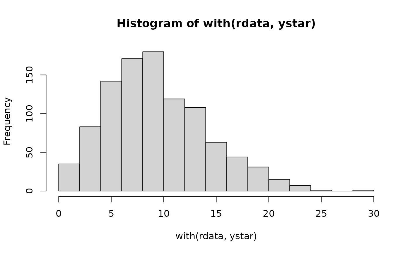
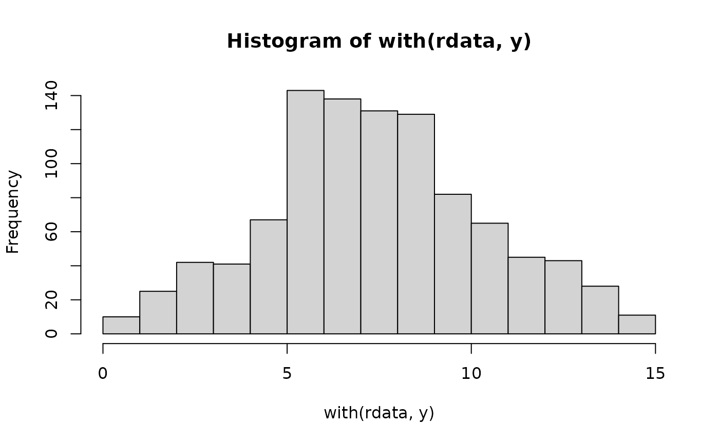
if (FALSE)  par(mfrow = c(1, 2))
hist(with(rdata, ystar)); hist(with(rdata, y))  # \dontrun{}


extra <- with(rdata, list(rightcensored = ystar > U))
fit <- vglm(y ~ 1, cens.rayleigh, data = rdata, trace = TRUE,
            extra = extra, crit = "coef")
#> Iteration 1: coefficients = 1.7723656
#> Iteration 2: coefficients = 1.9362991
#> Iteration 3: coefficients = 1.9863006
#> Iteration 4: coefficients = 2.0029459
#> Iteration 5: coefficients = 2.0086811
#> Iteration 6: coefficients = 2.0106812
#> Iteration 7: coefficients = 2.0113817
#> Iteration 8: coefficients = 2.0116274
#> Iteration 9: coefficients = 2.0117137
#> Iteration 10: coefficients = 2.0117439
#> Iteration 11: coefficients = 2.0117545
#> Iteration 12: coefficients = 2.0117583
#> Iteration 13: coefficients = 2.0117596
#> Iteration 14: coefficients = 2.01176
#> Iteration 15: coefficients = 2.0117602
table(fit@extra$rightcen)
#> 
#> FALSE  TRUE 
#>   571   429 
coef(fit, matrix = TRUE)
#>             loglink(scale)
#> (Intercept)        2.01176
head(fitted(fit))
#>      [,1]
#> 1 9.37036
#> 2 9.37036
#> 3 9.37036
#> 4 9.37036
#> 5 9.37036
#> 6 9.37036