Find the Highest Maximum A Posteriori probability estimate (MAP) of a
posterior, i.e., the value associated with the highest probability density
(the "peak" of the posterior distribution). In other words, it is an estimation
of the mode for continuous parameters. Note that this function relies on
estimate_density(), which by default uses a different smoothing bandwidth
("SJ") compared to the legacy default implemented the base R density()
function ("nrd0").
map_estimate(x, ...)

# S3 method for class 'numeric'
map_estimate(x, precision = 2^10, method = "kernel", verbose = TRUE, ...)

# S3 method for class 'brmsfit'
map_estimate(
  x,
  precision = 2^10,
  method = "kernel",
  effects = "fixed",
  component = "conditional",
  parameters = NULL,
  verbose = TRUE,
  ...
)

# S3 method for class 'data.frame'
map_estimate(
  x,
  precision = 2^10,
  method = "kernel",
  rvar_col = NULL,
  verbose = TRUE,
  ...
)

# S3 method for class 'get_predicted'
map_estimate(
  x,
  precision = 2^10,
  method = "kernel",
  use_iterations = FALSE,
  verbose = TRUE,
  ...
)
Arguments
- x
Vector representing a posterior distribution, or a data frame of such vectors. Can also be a Bayesian model. bayestestR supports a wide range of models (see, for example,
methods("hdi")) and not all of those are documented in the 'Usage' section, because methods for other classes mostly resemble the arguments of the.numericor.data.framemethods.- ...
Currently not used.
- precision
Number of points of density data. See the
nparameter indensity.- method
Density estimation method. Can be
"kernel"(default),"logspline"or"KernSmooth".- verbose
Toggle off warnings.
- effects
Should variables for fixed effects (
"fixed"), random effects ("random") or both ("all") be returned? Only applies to mixed models. May be abbreviated.For models of from packages brms or rstanarm there are additional options:
"fixed"returns fixed effects."random_variance"return random effects parameters (variance and correlation components, e.g. those parameters that start withsd_orcor_)."grouplevel"returns random effects group level estimates, i.e. those parameters that start withr_."random"returns both"random_variance"and"grouplevel"."all"returns fixed effects and random effects variances."full"returns all parameters.
- component
Which type of parameters to return, such as parameters for the conditional model, the zero-inflated part of the model, the dispersion term, etc. See details in section Model Components. May be abbreviated. Note that the conditional component also refers to the count or mean component - names may differ, depending on the modeling package. There are three convenient shortcuts (not applicable to all model classes):
component = "all"returns all possible parameters.If
component = "location", location parameters such asconditional,zero_inflated,smooth_terms, orinstrumentsare returned (everything that are fixed or random effects - depending on theeffectsargument - but no auxiliary parameters).For
component = "distributional"(or"auxiliary"), components likesigma,dispersion,betaorprecision(and other auxiliary parameters) are returned.
- parameters
Regular expression pattern that describes the parameters that should be returned. Meta-parameters (like
lp__orprior_) are filtered by default, so only parameters that typically appear in thesummary()are returned. Useparametersto select specific parameters for the output.- rvar_col
A single character - the name of an
rvarcolumn in the data frame to be processed. See example inp_direction().- use_iterations
Logical, if
TRUEandxis aget_predictedobject, (returned byinsight::get_predicted()), the function is applied to the iterations instead of the predictions. This only applies to models that return iterations for predicted values (e.g.,brmsfitmodels).
Value
A numeric value if x is a vector. If x is a model-object,
returns a data frame with following columns:
Parameter: The model parameter(s), ifxis a model-object. Ifxis a vector, this column is missing.MAP_Estimate: The MAP estimate for the posterior or each model parameter.
Model components
Possible values for the component argument depend on the model class.
Following are valid options:
"all": returns all model components, applies to all models, but will only have an effect for models with more than just the conditional model component."conditional": only returns the conditional component, i.e. "fixed effects" terms from the model. Will only have an effect for models with more than just the conditional model component."smooth_terms": returns smooth terms, only applies to GAMs (or similar models that may contain smooth terms)."zero_inflated"(or"zi"): returns the zero-inflation component."location": returns location parameters such asconditional,zero_inflated, orsmooth_terms(everything that are fixed or random effects - depending on theeffectsargument - but no auxiliary parameters)."distributional"(or"auxiliary"): components likesigma,dispersion,betaorprecision(and other auxiliary parameters) are returned.
For models of class brmsfit (package brms), even more options are
possible for the component argument, which are not all documented in detail
here. See also ?insight::find_parameters.
Examples
# \donttest{
library(bayestestR)
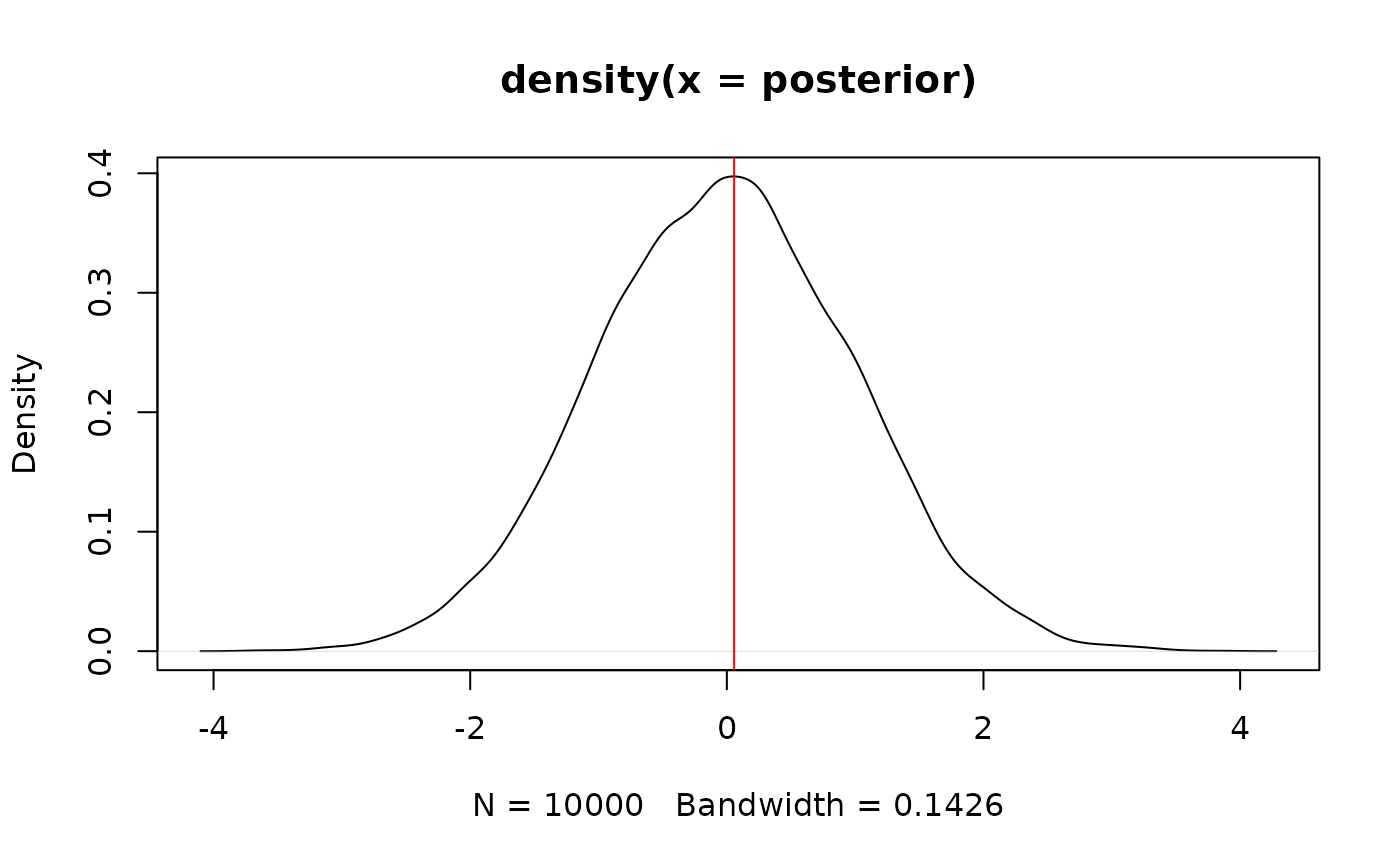
posterior <- rnorm(10000)
map_estimate(posterior)
#> MAP Estimate
#>
#> Parameter | MAP_Estimate
#> ------------------------
#> x | 0.06
plot(density(posterior))
abline(v = as.numeric(map_estimate(posterior)), col = "red")
 model <- rstanarm::stan_glm(mpg ~ wt + cyl, data = mtcars)
#>
#> SAMPLING FOR MODEL 'continuous' NOW (CHAIN 1).
#> Chain 1:
#> Chain 1: Gradient evaluation took 3.1e-05 seconds
#> Chain 1: 1000 transitions using 10 leapfrog steps per transition would take 0.31 seconds.
#> Chain 1: Adjust your expectations accordingly!
#> Chain 1:
#> Chain 1:
#> Chain 1: Iteration: 1 / 2000 [ 0%] (Warmup)
#> Chain 1: Iteration: 200 / 2000 [ 10%] (Warmup)
#> Chain 1: Iteration: 400 / 2000 [ 20%] (Warmup)
#> Chain 1: Iteration: 600 / 2000 [ 30%] (Warmup)
#> Chain 1: Iteration: 800 / 2000 [ 40%] (Warmup)
#> Chain 1: Iteration: 1000 / 2000 [ 50%] (Warmup)
#> Chain 1: Iteration: 1001 / 2000 [ 50%] (Sampling)
#> Chain 1: Iteration: 1200 / 2000 [ 60%] (Sampling)
#> Chain 1: Iteration: 1400 / 2000 [ 70%] (Sampling)
#> Chain 1: Iteration: 1600 / 2000 [ 80%] (Sampling)
#> Chain 1: Iteration: 1800 / 2000 [ 90%] (Sampling)
#> Chain 1: Iteration: 2000 / 2000 [100%] (Sampling)
#> Chain 1:
#> Chain 1: Elapsed Time: 0.059 seconds (Warm-up)
#> Chain 1: 0.043 seconds (Sampling)
#> Chain 1: 0.102 seconds (Total)
#> Chain 1:
#>
#> SAMPLING FOR MODEL 'continuous' NOW (CHAIN 2).
#> Chain 2:
#> Chain 2: Gradient evaluation took 1.3e-05 seconds
#> Chain 2: 1000 transitions using 10 leapfrog steps per transition would take 0.13 seconds.
#> Chain 2: Adjust your expectations accordingly!
#> Chain 2:
#> Chain 2:
#> Chain 2: Iteration: 1 / 2000 [ 0%] (Warmup)
#> Chain 2: Iteration: 200 / 2000 [ 10%] (Warmup)
#> Chain 2: Iteration: 400 / 2000 [ 20%] (Warmup)
#> Chain 2: Iteration: 600 / 2000 [ 30%] (Warmup)
#> Chain 2: Iteration: 800 / 2000 [ 40%] (Warmup)
#> Chain 2: Iteration: 1000 / 2000 [ 50%] (Warmup)
#> Chain 2: Iteration: 1001 / 2000 [ 50%] (Sampling)
#> Chain 2: Iteration: 1200 / 2000 [ 60%] (Sampling)
#> Chain 2: Iteration: 1400 / 2000 [ 70%] (Sampling)
#> Chain 2: Iteration: 1600 / 2000 [ 80%] (Sampling)
#> Chain 2: Iteration: 1800 / 2000 [ 90%] (Sampling)
#> Chain 2: Iteration: 2000 / 2000 [100%] (Sampling)
#> Chain 2:
#> Chain 2: Elapsed Time: 0.048 seconds (Warm-up)
#> Chain 2: 0.062 seconds (Sampling)
#> Chain 2: 0.11 seconds (Total)
#> Chain 2:
#>
#> SAMPLING FOR MODEL 'continuous' NOW (CHAIN 3).
#> Chain 3:
#> Chain 3: Gradient evaluation took 1.5e-05 seconds
#> Chain 3: 1000 transitions using 10 leapfrog steps per transition would take 0.15 seconds.
#> Chain 3: Adjust your expectations accordingly!
#> Chain 3:
#> Chain 3:
#> Chain 3: Iteration: 1 / 2000 [ 0%] (Warmup)
#> Chain 3: Iteration: 200 / 2000 [ 10%] (Warmup)
#> Chain 3: Iteration: 400 / 2000 [ 20%] (Warmup)
#> Chain 3: Iteration: 600 / 2000 [ 30%] (Warmup)
#> Chain 3: Iteration: 800 / 2000 [ 40%] (Warmup)
#> Chain 3: Iteration: 1000 / 2000 [ 50%] (Warmup)
#> Chain 3: Iteration: 1001 / 2000 [ 50%] (Sampling)
#> Chain 3: Iteration: 1200 / 2000 [ 60%] (Sampling)
#> Chain 3: Iteration: 1400 / 2000 [ 70%] (Sampling)
#> Chain 3: Iteration: 1600 / 2000 [ 80%] (Sampling)
#> Chain 3: Iteration: 1800 / 2000 [ 90%] (Sampling)
#> Chain 3: Iteration: 2000 / 2000 [100%] (Sampling)
#> Chain 3:
#> Chain 3: Elapsed Time: 0.077 seconds (Warm-up)
#> Chain 3: 0.07 seconds (Sampling)
#> Chain 3: 0.147 seconds (Total)
#> Chain 3:
#>
#> SAMPLING FOR MODEL 'continuous' NOW (CHAIN 4).
#> Chain 4:
#> Chain 4: Gradient evaluation took 1.7e-05 seconds
#> Chain 4: 1000 transitions using 10 leapfrog steps per transition would take 0.17 seconds.
#> Chain 4: Adjust your expectations accordingly!
#> Chain 4:
#> Chain 4:
#> Chain 4: Iteration: 1 / 2000 [ 0%] (Warmup)
#> Chain 4: Iteration: 200 / 2000 [ 10%] (Warmup)
#> Chain 4: Iteration: 400 / 2000 [ 20%] (Warmup)
#> Chain 4: Iteration: 600 / 2000 [ 30%] (Warmup)
#> Chain 4: Iteration: 800 / 2000 [ 40%] (Warmup)
#> Chain 4: Iteration: 1000 / 2000 [ 50%] (Warmup)
#> Chain 4: Iteration: 1001 / 2000 [ 50%] (Sampling)
#> Chain 4: Iteration: 1200 / 2000 [ 60%] (Sampling)
#> Chain 4: Iteration: 1400 / 2000 [ 70%] (Sampling)
#> Chain 4: Iteration: 1600 / 2000 [ 80%] (Sampling)
#> Chain 4: Iteration: 1800 / 2000 [ 90%] (Sampling)
#> Chain 4: Iteration: 2000 / 2000 [100%] (Sampling)
#> Chain 4:
#> Chain 4: Elapsed Time: 0.074 seconds (Warm-up)
#> Chain 4: 0.074 seconds (Sampling)
#> Chain 4: 0.148 seconds (Total)
#> Chain 4:
map_estimate(model)
#> MAP Estimate
#>
#> Parameter | MAP_Estimate
#> --------------------------
#> (Intercept) | 39.82
#> wt | -3.13
#> cyl | -1.53
model <- brms::brm(mpg ~ wt + cyl, data = mtcars)
#> Compiling Stan program...
#> Start sampling
#>
#> SAMPLING FOR MODEL 'anon_model' NOW (CHAIN 1).
#> Chain 1:
#> Chain 1: Gradient evaluation took 1.1e-05 seconds
#> Chain 1: 1000 transitions using 10 leapfrog steps per transition would take 0.11 seconds.
#> Chain 1: Adjust your expectations accordingly!
#> Chain 1:
#> Chain 1:
#> Chain 1: Iteration: 1 / 2000 [ 0%] (Warmup)
#> Chain 1: Iteration: 200 / 2000 [ 10%] (Warmup)
#> Chain 1: Iteration: 400 / 2000 [ 20%] (Warmup)
#> Chain 1: Iteration: 600 / 2000 [ 30%] (Warmup)
#> Chain 1: Iteration: 800 / 2000 [ 40%] (Warmup)
#> Chain 1: Iteration: 1000 / 2000 [ 50%] (Warmup)
#> Chain 1: Iteration: 1001 / 2000 [ 50%] (Sampling)
#> Chain 1: Iteration: 1200 / 2000 [ 60%] (Sampling)
#> Chain 1: Iteration: 1400 / 2000 [ 70%] (Sampling)
#> Chain 1: Iteration: 1600 / 2000 [ 80%] (Sampling)
#> Chain 1: Iteration: 1800 / 2000 [ 90%] (Sampling)
#> Chain 1: Iteration: 2000 / 2000 [100%] (Sampling)
#> Chain 1:
#> Chain 1: Elapsed Time: 0.016 seconds (Warm-up)
#> Chain 1: 0.015 seconds (Sampling)
#> Chain 1: 0.031 seconds (Total)
#> Chain 1:
#>
#> SAMPLING FOR MODEL 'anon_model' NOW (CHAIN 2).
#> Chain 2:
#> Chain 2: Gradient evaluation took 4e-06 seconds
#> Chain 2: 1000 transitions using 10 leapfrog steps per transition would take 0.04 seconds.
#> Chain 2: Adjust your expectations accordingly!
#> Chain 2:
#> Chain 2:
#> Chain 2: Iteration: 1 / 2000 [ 0%] (Warmup)
#> Chain 2: Iteration: 200 / 2000 [ 10%] (Warmup)
#> Chain 2: Iteration: 400 / 2000 [ 20%] (Warmup)
#> Chain 2: Iteration: 600 / 2000 [ 30%] (Warmup)
#> Chain 2: Iteration: 800 / 2000 [ 40%] (Warmup)
#> Chain 2: Iteration: 1000 / 2000 [ 50%] (Warmup)
#> Chain 2: Iteration: 1001 / 2000 [ 50%] (Sampling)
#> Chain 2: Iteration: 1200 / 2000 [ 60%] (Sampling)
#> Chain 2: Iteration: 1400 / 2000 [ 70%] (Sampling)
#> Chain 2: Iteration: 1600 / 2000 [ 80%] (Sampling)
#> Chain 2: Iteration: 1800 / 2000 [ 90%] (Sampling)
#> Chain 2: Iteration: 2000 / 2000 [100%] (Sampling)
#> Chain 2:
#> Chain 2: Elapsed Time: 0.017 seconds (Warm-up)
#> Chain 2: 0.016 seconds (Sampling)
#> Chain 2: 0.033 seconds (Total)
#> Chain 2:
#>
#> SAMPLING FOR MODEL 'anon_model' NOW (CHAIN 3).
#> Chain 3:
#> Chain 3: Gradient evaluation took 5e-06 seconds
#> Chain 3: 1000 transitions using 10 leapfrog steps per transition would take 0.05 seconds.
#> Chain 3: Adjust your expectations accordingly!
#> Chain 3:
#> Chain 3:
#> Chain 3: Iteration: 1 / 2000 [ 0%] (Warmup)
#> Chain 3: Iteration: 200 / 2000 [ 10%] (Warmup)
#> Chain 3: Iteration: 400 / 2000 [ 20%] (Warmup)
#> Chain 3: Iteration: 600 / 2000 [ 30%] (Warmup)
#> Chain 3: Iteration: 800 / 2000 [ 40%] (Warmup)
#> Chain 3: Iteration: 1000 / 2000 [ 50%] (Warmup)
#> Chain 3: Iteration: 1001 / 2000 [ 50%] (Sampling)
#> Chain 3: Iteration: 1200 / 2000 [ 60%] (Sampling)
#> Chain 3: Iteration: 1400 / 2000 [ 70%] (Sampling)
#> Chain 3: Iteration: 1600 / 2000 [ 80%] (Sampling)
#> Chain 3: Iteration: 1800 / 2000 [ 90%] (Sampling)
#> Chain 3: Iteration: 2000 / 2000 [100%] (Sampling)
#> Chain 3:
#> Chain 3: Elapsed Time: 0.018 seconds (Warm-up)
#> Chain 3: 0.015 seconds (Sampling)
#> Chain 3: 0.033 seconds (Total)
#> Chain 3:
#>
#> SAMPLING FOR MODEL 'anon_model' NOW (CHAIN 4).
#> Chain 4:
#> Chain 4: Gradient evaluation took 4e-06 seconds
#> Chain 4: 1000 transitions using 10 leapfrog steps per transition would take 0.04 seconds.
#> Chain 4: Adjust your expectations accordingly!
#> Chain 4:
#> Chain 4:
#> Chain 4: Iteration: 1 / 2000 [ 0%] (Warmup)
#> Chain 4: Iteration: 200 / 2000 [ 10%] (Warmup)
#> Chain 4: Iteration: 400 / 2000 [ 20%] (Warmup)
#> Chain 4: Iteration: 600 / 2000 [ 30%] (Warmup)
#> Chain 4: Iteration: 800 / 2000 [ 40%] (Warmup)
#> Chain 4: Iteration: 1000 / 2000 [ 50%] (Warmup)
#> Chain 4: Iteration: 1001 / 2000 [ 50%] (Sampling)
#> Chain 4: Iteration: 1200 / 2000 [ 60%] (Sampling)
#> Chain 4: Iteration: 1400 / 2000 [ 70%] (Sampling)
#> Chain 4: Iteration: 1600 / 2000 [ 80%] (Sampling)
#> Chain 4: Iteration: 1800 / 2000 [ 90%] (Sampling)
#> Chain 4: Iteration: 2000 / 2000 [100%] (Sampling)
#> Chain 4:
#> Chain 4: Elapsed Time: 0.018 seconds (Warm-up)
#> Chain 4: 0.017 seconds (Sampling)
#> Chain 4: 0.035 seconds (Total)
#> Chain 4:
map_estimate(model)
#> MAP Estimate
#>
#> Parameter | MAP_Estimate
#> --------------------------
#> b_Intercept | 39.67
#> b_wt | -3.06
#> b_cyl | -1.58
# }
model <- rstanarm::stan_glm(mpg ~ wt + cyl, data = mtcars)
#>
#> SAMPLING FOR MODEL 'continuous' NOW (CHAIN 1).
#> Chain 1:
#> Chain 1: Gradient evaluation took 3.1e-05 seconds
#> Chain 1: 1000 transitions using 10 leapfrog steps per transition would take 0.31 seconds.
#> Chain 1: Adjust your expectations accordingly!
#> Chain 1:
#> Chain 1:
#> Chain 1: Iteration: 1 / 2000 [ 0%] (Warmup)
#> Chain 1: Iteration: 200 / 2000 [ 10%] (Warmup)
#> Chain 1: Iteration: 400 / 2000 [ 20%] (Warmup)
#> Chain 1: Iteration: 600 / 2000 [ 30%] (Warmup)
#> Chain 1: Iteration: 800 / 2000 [ 40%] (Warmup)
#> Chain 1: Iteration: 1000 / 2000 [ 50%] (Warmup)
#> Chain 1: Iteration: 1001 / 2000 [ 50%] (Sampling)
#> Chain 1: Iteration: 1200 / 2000 [ 60%] (Sampling)
#> Chain 1: Iteration: 1400 / 2000 [ 70%] (Sampling)
#> Chain 1: Iteration: 1600 / 2000 [ 80%] (Sampling)
#> Chain 1: Iteration: 1800 / 2000 [ 90%] (Sampling)
#> Chain 1: Iteration: 2000 / 2000 [100%] (Sampling)
#> Chain 1:
#> Chain 1: Elapsed Time: 0.059 seconds (Warm-up)
#> Chain 1: 0.043 seconds (Sampling)
#> Chain 1: 0.102 seconds (Total)
#> Chain 1:
#>
#> SAMPLING FOR MODEL 'continuous' NOW (CHAIN 2).
#> Chain 2:
#> Chain 2: Gradient evaluation took 1.3e-05 seconds
#> Chain 2: 1000 transitions using 10 leapfrog steps per transition would take 0.13 seconds.
#> Chain 2: Adjust your expectations accordingly!
#> Chain 2:
#> Chain 2:
#> Chain 2: Iteration: 1 / 2000 [ 0%] (Warmup)
#> Chain 2: Iteration: 200 / 2000 [ 10%] (Warmup)
#> Chain 2: Iteration: 400 / 2000 [ 20%] (Warmup)
#> Chain 2: Iteration: 600 / 2000 [ 30%] (Warmup)
#> Chain 2: Iteration: 800 / 2000 [ 40%] (Warmup)
#> Chain 2: Iteration: 1000 / 2000 [ 50%] (Warmup)
#> Chain 2: Iteration: 1001 / 2000 [ 50%] (Sampling)
#> Chain 2: Iteration: 1200 / 2000 [ 60%] (Sampling)
#> Chain 2: Iteration: 1400 / 2000 [ 70%] (Sampling)
#> Chain 2: Iteration: 1600 / 2000 [ 80%] (Sampling)
#> Chain 2: Iteration: 1800 / 2000 [ 90%] (Sampling)
#> Chain 2: Iteration: 2000 / 2000 [100%] (Sampling)
#> Chain 2:
#> Chain 2: Elapsed Time: 0.048 seconds (Warm-up)
#> Chain 2: 0.062 seconds (Sampling)
#> Chain 2: 0.11 seconds (Total)
#> Chain 2:
#>
#> SAMPLING FOR MODEL 'continuous' NOW (CHAIN 3).
#> Chain 3:
#> Chain 3: Gradient evaluation took 1.5e-05 seconds
#> Chain 3: 1000 transitions using 10 leapfrog steps per transition would take 0.15 seconds.
#> Chain 3: Adjust your expectations accordingly!
#> Chain 3:
#> Chain 3:
#> Chain 3: Iteration: 1 / 2000 [ 0%] (Warmup)
#> Chain 3: Iteration: 200 / 2000 [ 10%] (Warmup)
#> Chain 3: Iteration: 400 / 2000 [ 20%] (Warmup)
#> Chain 3: Iteration: 600 / 2000 [ 30%] (Warmup)
#> Chain 3: Iteration: 800 / 2000 [ 40%] (Warmup)
#> Chain 3: Iteration: 1000 / 2000 [ 50%] (Warmup)
#> Chain 3: Iteration: 1001 / 2000 [ 50%] (Sampling)
#> Chain 3: Iteration: 1200 / 2000 [ 60%] (Sampling)
#> Chain 3: Iteration: 1400 / 2000 [ 70%] (Sampling)
#> Chain 3: Iteration: 1600 / 2000 [ 80%] (Sampling)
#> Chain 3: Iteration: 1800 / 2000 [ 90%] (Sampling)
#> Chain 3: Iteration: 2000 / 2000 [100%] (Sampling)
#> Chain 3:
#> Chain 3: Elapsed Time: 0.077 seconds (Warm-up)
#> Chain 3: 0.07 seconds (Sampling)
#> Chain 3: 0.147 seconds (Total)
#> Chain 3:
#>
#> SAMPLING FOR MODEL 'continuous' NOW (CHAIN 4).
#> Chain 4:
#> Chain 4: Gradient evaluation took 1.7e-05 seconds
#> Chain 4: 1000 transitions using 10 leapfrog steps per transition would take 0.17 seconds.
#> Chain 4: Adjust your expectations accordingly!
#> Chain 4:
#> Chain 4:
#> Chain 4: Iteration: 1 / 2000 [ 0%] (Warmup)
#> Chain 4: Iteration: 200 / 2000 [ 10%] (Warmup)
#> Chain 4: Iteration: 400 / 2000 [ 20%] (Warmup)
#> Chain 4: Iteration: 600 / 2000 [ 30%] (Warmup)
#> Chain 4: Iteration: 800 / 2000 [ 40%] (Warmup)
#> Chain 4: Iteration: 1000 / 2000 [ 50%] (Warmup)
#> Chain 4: Iteration: 1001 / 2000 [ 50%] (Sampling)
#> Chain 4: Iteration: 1200 / 2000 [ 60%] (Sampling)
#> Chain 4: Iteration: 1400 / 2000 [ 70%] (Sampling)
#> Chain 4: Iteration: 1600 / 2000 [ 80%] (Sampling)
#> Chain 4: Iteration: 1800 / 2000 [ 90%] (Sampling)
#> Chain 4: Iteration: 2000 / 2000 [100%] (Sampling)
#> Chain 4:
#> Chain 4: Elapsed Time: 0.074 seconds (Warm-up)
#> Chain 4: 0.074 seconds (Sampling)
#> Chain 4: 0.148 seconds (Total)
#> Chain 4:
map_estimate(model)
#> MAP Estimate
#>
#> Parameter | MAP_Estimate
#> --------------------------
#> (Intercept) | 39.82
#> wt | -3.13
#> cyl | -1.53
model <- brms::brm(mpg ~ wt + cyl, data = mtcars)
#> Compiling Stan program...
#> Start sampling
#>
#> SAMPLING FOR MODEL 'anon_model' NOW (CHAIN 1).
#> Chain 1:
#> Chain 1: Gradient evaluation took 1.1e-05 seconds
#> Chain 1: 1000 transitions using 10 leapfrog steps per transition would take 0.11 seconds.
#> Chain 1: Adjust your expectations accordingly!
#> Chain 1:
#> Chain 1:
#> Chain 1: Iteration: 1 / 2000 [ 0%] (Warmup)
#> Chain 1: Iteration: 200 / 2000 [ 10%] (Warmup)
#> Chain 1: Iteration: 400 / 2000 [ 20%] (Warmup)
#> Chain 1: Iteration: 600 / 2000 [ 30%] (Warmup)
#> Chain 1: Iteration: 800 / 2000 [ 40%] (Warmup)
#> Chain 1: Iteration: 1000 / 2000 [ 50%] (Warmup)
#> Chain 1: Iteration: 1001 / 2000 [ 50%] (Sampling)
#> Chain 1: Iteration: 1200 / 2000 [ 60%] (Sampling)
#> Chain 1: Iteration: 1400 / 2000 [ 70%] (Sampling)
#> Chain 1: Iteration: 1600 / 2000 [ 80%] (Sampling)
#> Chain 1: Iteration: 1800 / 2000 [ 90%] (Sampling)
#> Chain 1: Iteration: 2000 / 2000 [100%] (Sampling)
#> Chain 1:
#> Chain 1: Elapsed Time: 0.016 seconds (Warm-up)
#> Chain 1: 0.015 seconds (Sampling)
#> Chain 1: 0.031 seconds (Total)
#> Chain 1:
#>
#> SAMPLING FOR MODEL 'anon_model' NOW (CHAIN 2).
#> Chain 2:
#> Chain 2: Gradient evaluation took 4e-06 seconds
#> Chain 2: 1000 transitions using 10 leapfrog steps per transition would take 0.04 seconds.
#> Chain 2: Adjust your expectations accordingly!
#> Chain 2:
#> Chain 2:
#> Chain 2: Iteration: 1 / 2000 [ 0%] (Warmup)
#> Chain 2: Iteration: 200 / 2000 [ 10%] (Warmup)
#> Chain 2: Iteration: 400 / 2000 [ 20%] (Warmup)
#> Chain 2: Iteration: 600 / 2000 [ 30%] (Warmup)
#> Chain 2: Iteration: 800 / 2000 [ 40%] (Warmup)
#> Chain 2: Iteration: 1000 / 2000 [ 50%] (Warmup)
#> Chain 2: Iteration: 1001 / 2000 [ 50%] (Sampling)
#> Chain 2: Iteration: 1200 / 2000 [ 60%] (Sampling)
#> Chain 2: Iteration: 1400 / 2000 [ 70%] (Sampling)
#> Chain 2: Iteration: 1600 / 2000 [ 80%] (Sampling)
#> Chain 2: Iteration: 1800 / 2000 [ 90%] (Sampling)
#> Chain 2: Iteration: 2000 / 2000 [100%] (Sampling)
#> Chain 2:
#> Chain 2: Elapsed Time: 0.017 seconds (Warm-up)
#> Chain 2: 0.016 seconds (Sampling)
#> Chain 2: 0.033 seconds (Total)
#> Chain 2:
#>
#> SAMPLING FOR MODEL 'anon_model' NOW (CHAIN 3).
#> Chain 3:
#> Chain 3: Gradient evaluation took 5e-06 seconds
#> Chain 3: 1000 transitions using 10 leapfrog steps per transition would take 0.05 seconds.
#> Chain 3: Adjust your expectations accordingly!
#> Chain 3:
#> Chain 3:
#> Chain 3: Iteration: 1 / 2000 [ 0%] (Warmup)
#> Chain 3: Iteration: 200 / 2000 [ 10%] (Warmup)
#> Chain 3: Iteration: 400 / 2000 [ 20%] (Warmup)
#> Chain 3: Iteration: 600 / 2000 [ 30%] (Warmup)
#> Chain 3: Iteration: 800 / 2000 [ 40%] (Warmup)
#> Chain 3: Iteration: 1000 / 2000 [ 50%] (Warmup)
#> Chain 3: Iteration: 1001 / 2000 [ 50%] (Sampling)
#> Chain 3: Iteration: 1200 / 2000 [ 60%] (Sampling)
#> Chain 3: Iteration: 1400 / 2000 [ 70%] (Sampling)
#> Chain 3: Iteration: 1600 / 2000 [ 80%] (Sampling)
#> Chain 3: Iteration: 1800 / 2000 [ 90%] (Sampling)
#> Chain 3: Iteration: 2000 / 2000 [100%] (Sampling)
#> Chain 3:
#> Chain 3: Elapsed Time: 0.018 seconds (Warm-up)
#> Chain 3: 0.015 seconds (Sampling)
#> Chain 3: 0.033 seconds (Total)
#> Chain 3:
#>
#> SAMPLING FOR MODEL 'anon_model' NOW (CHAIN 4).
#> Chain 4:
#> Chain 4: Gradient evaluation took 4e-06 seconds
#> Chain 4: 1000 transitions using 10 leapfrog steps per transition would take 0.04 seconds.
#> Chain 4: Adjust your expectations accordingly!
#> Chain 4:
#> Chain 4:
#> Chain 4: Iteration: 1 / 2000 [ 0%] (Warmup)
#> Chain 4: Iteration: 200 / 2000 [ 10%] (Warmup)
#> Chain 4: Iteration: 400 / 2000 [ 20%] (Warmup)
#> Chain 4: Iteration: 600 / 2000 [ 30%] (Warmup)
#> Chain 4: Iteration: 800 / 2000 [ 40%] (Warmup)
#> Chain 4: Iteration: 1000 / 2000 [ 50%] (Warmup)
#> Chain 4: Iteration: 1001 / 2000 [ 50%] (Sampling)
#> Chain 4: Iteration: 1200 / 2000 [ 60%] (Sampling)
#> Chain 4: Iteration: 1400 / 2000 [ 70%] (Sampling)
#> Chain 4: Iteration: 1600 / 2000 [ 80%] (Sampling)
#> Chain 4: Iteration: 1800 / 2000 [ 90%] (Sampling)
#> Chain 4: Iteration: 2000 / 2000 [100%] (Sampling)
#> Chain 4:
#> Chain 4: Elapsed Time: 0.018 seconds (Warm-up)
#> Chain 4: 0.017 seconds (Sampling)
#> Chain 4: 0.035 seconds (Total)
#> Chain 4:
map_estimate(model)
#> MAP Estimate
#>
#> Parameter | MAP_Estimate
#> --------------------------
#> b_Intercept | 39.67
#> b_wt | -3.06
#> b_cyl | -1.58
# }