Create a Beta Regression Distribution

Class and methods for beta distributions in regression specification using the workflow from the distributions3 package.

Usage

BetaR(mu = numeric(), phi = numeric())

Arguments

mu: numeric. The mean of the beta distribution.
phi: numeric. The precision parameter of the beta distribution.

Details

Alternative parameterization of the classic beta distribution in terms of its mean mu and precision parameter phi. Thus, the distribution provided by BetaR is equivalent to the Beta distribution with parameters alpha = mu * phi and beta = (1 - mu) * phi.

Value

A BetaR distribution object.

Examples

## package and random seed
library("distributions3")
set.seed(6020)

## three beta distributions
X <- BetaR(
  mu  = c(0.25, 0.50, 0.75),
  phi = c(1, 1, 2)
)
# \donttest{
X
#> [1] "BetaR(mu = 0.25, phi = 1)" "BetaR(mu = 0.50, phi = 1)"
#> [3] "BetaR(mu = 0.75, phi = 2)"

## compute moments of the distribution
mean(X)
#> [1] 0.25 0.50 0.75
variance(X)
#> [1] 0.09375 0.12500 0.06250
skewness(X)
#> [1] -0.1666667 -1.5000000  0.0000000
kurtosis(X)
#> [1] -0.1666667 -1.5000000  0.0000000

## support interval (minimum and maximum)
support(X)
#>      min max
#> [1,]   0   1
#> [2,]   0   1
#> [3,]   0   1

## simulate random variables
random(X, 5)
#>            r_1       r_2         r_3       r_4        r_5
#> [1,] 0.7497152 0.8385523 0.031967958 0.9188288 0.54543668
#> [2,] 0.1886452 0.9982310 0.004743561 0.1429292 0.07917131
#> [3,] 0.9569594 0.9906614 0.757365599 0.9186620 0.84031674

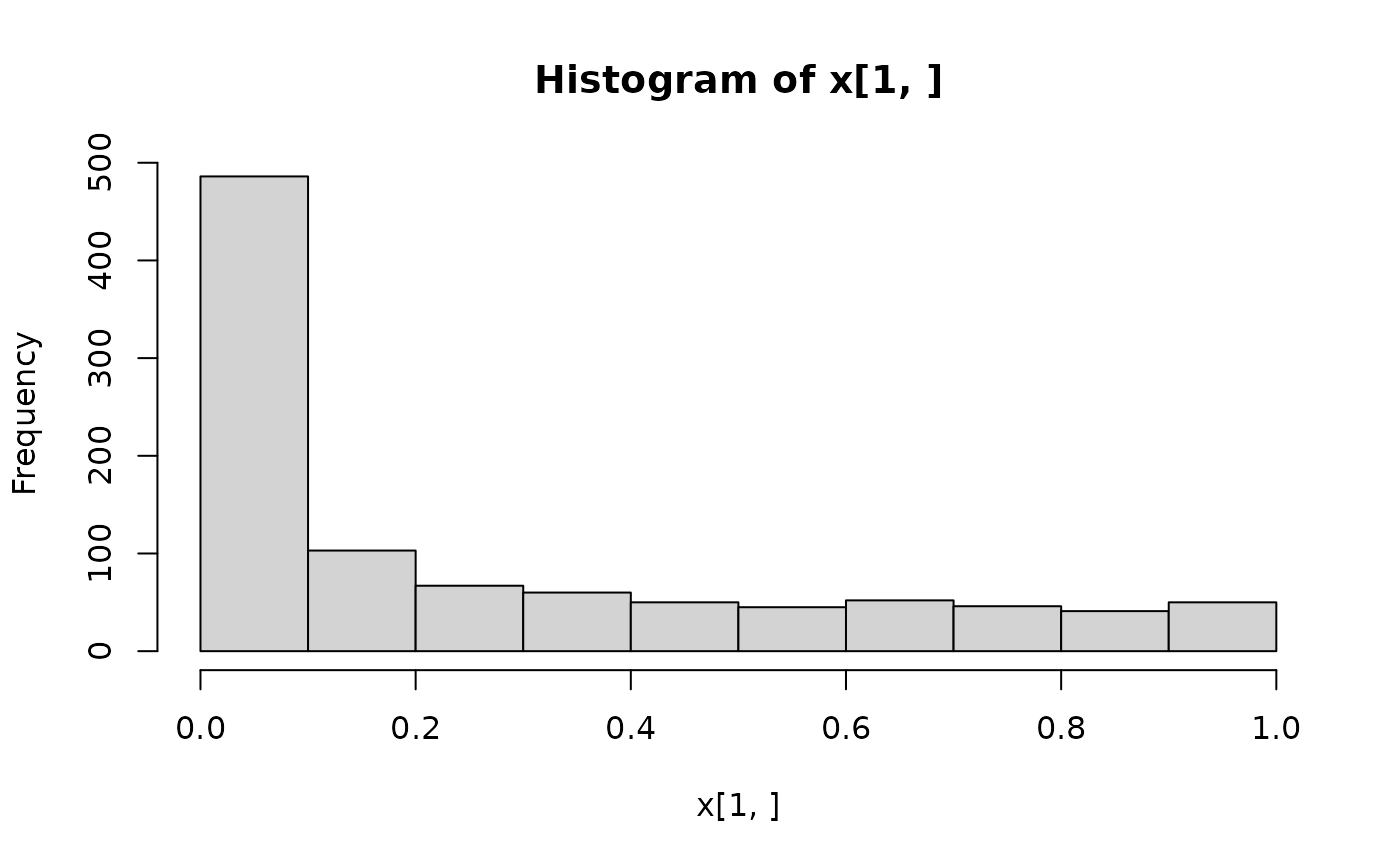
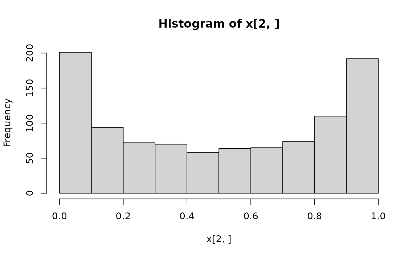
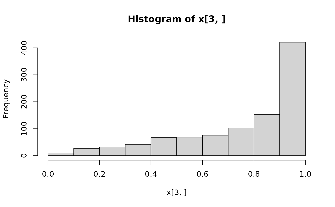
## histograms of 1,000 simulated observations
x <- random(X, 1000)
hist(x[1, ])

hist(x[2, ])

hist(x[3, ])


## probability density function (PDF) and log-density (or log-likelihood)
x <- c(0.25, 0.5, 0.75)
pdf(X, x)
#> [1] 0.6840925 0.6366198 1.1026578
pdf(X, x, log = TRUE)
#> [1] -0.37966219 -0.45158271  0.09772344
log_pdf(X, x)
#> [1] -0.37966219 -0.45158271  0.09772344

## cumulative distribution function (CDF)
cdf(X, x)
#> [1] 0.6453748 0.5000000 0.3910022

## quantiles
quantile(X, 0.5)
#> [1] 0.09331223 0.50000000 0.83680601

## cdf() and quantile() are inverses (except at censoring points)
cdf(X, quantile(X, 0.5))
#> [1] 0.5 0.5 0.5
quantile(X, cdf(X, 1))
#> [1] 1 1 1

## all methods above can either be applied elementwise or for
## all combinations of X and x, if length(X) = length(x),
## also the result can be assured to be a matrix via drop = FALSE
p <- c(0.05, 0.5, 0.95)
quantile(X, p, elementwise = FALSE)
#>            q_0.05      q_0.5    q_0.95
#> [1,] 9.512588e-06 0.09331223 0.9118445
#> [2,] 6.155830e-03 0.50000000 0.9938442
#> [3,] 2.285198e-01 0.83680601 0.9984571
quantile(X, p, elementwise = TRUE)
#> [1] 9.512588e-06 5.000000e-01 9.984571e-01
quantile(X, p, elementwise = TRUE, drop = FALSE)
#>          quantile
#> [1,] 9.512588e-06
#> [2,] 5.000000e-01
#> [3,] 9.984571e-01

## compare theoretical and empirical mean from 1,000 simulated observations
cbind(
  "theoretical" = mean(X),
  "empirical" = rowMeans(random(X, 1000))
)
#>      theoretical empirical
#> [1,]        0.25 0.2464581
#> [2,]        0.50 0.4941967
#> [3,]        0.75 0.7542970
# }