Estimation of Gasoline Yields from Crude Oil
GasolineYield.RdOperational data of the proportion of crude oil converted to gasoline after distillation and fractionation.
Usage
data("GasolineYield", package = "betareg")Format
A data frame containing 32 observations on 6 variables.
- yield
proportion of crude oil converted to gasoline after distillation and fractionation.
- gravity
crude oil gravity (degrees API).
- pressure
vapor pressure of crude oil (lbf/in2).
- temp10
temperature (degrees F) at which 10 percent of crude oil has vaporized.
- temp
temperature (degrees F) at which all gasoline has vaporized.
- batch
factor indicating unique batch of conditions
gravity,pressure, andtemp10.
Details
This dataset was collected by Prater (1956), its dependent variable is the proportion of crude oil after distillation and fractionation. This dataset was analyzed by Atkinson (1985), who used the linear regression model and noted that there is “indication that the error distribution is not quite symmetrical, giving rise to some unduly large and small residuals” (p. 60).
The dataset contains 32 observations on the response and on the independent
variables. It has been noted (Daniel and Wood, 1971, Chapter 8) that there are only
ten sets of values of the first three explanatory variables which correspond to
ten different crudes and were subjected to experimentally controlled distillation
conditions. These conditions are captured in variable batch and
the data were ordered according to the ascending order of temp10.
References
Atkinson, A.C. (1985). Plots, Transformations and Regression: An Introduction to Graphical Methods of Diagnostic Regression Analysis. New York: Oxford University Press.
Cribari-Neto, F., and Zeileis, A. (2010). Beta Regression in R. Journal of Statistical Software, 34(2), 1–24. doi:10.18637/jss.v034.i02
Daniel, C., and Wood, F.S. (1971). Fitting Equations to Data. New York: John Wiley and Sons.
Ferrari, S.L.P., and Cribari-Neto, F. (2004). Beta Regression for Modeling Rates and Proportions. Journal of Applied Statistics, 31(7), 799–815.
Prater, N.H. (1956). Estimate Gasoline Yields from Crudes. Petroleum Refiner, 35(5), 236–238.
Examples
## IGNORE_RDIFF_BEGIN
data("GasolineYield", package = "betareg")
gy1 <- betareg(yield ~ gravity + pressure + temp10 + temp, data = GasolineYield)
summary(gy1)
#>
#> Call:
#> betareg(formula = yield ~ gravity + pressure + temp10 + temp, data = GasolineYield)
#>
#> Quantile residuals:
#> Min 1Q Median 3Q Max
#> -1.9010 -0.6829 -0.0385 0.5531 2.1314
#>
#> Coefficients (mean model with logit link):
#> Estimate Std. Error z value Pr(>|z|)
#> (Intercept) -2.6949422 0.7625693 -3.534 0.000409 ***
#> gravity 0.0045412 0.0071419 0.636 0.524871
#> pressure 0.0304135 0.0281007 1.082 0.279117
#> temp10 -0.0110449 0.0022640 -4.879 1.07e-06 ***
#> temp 0.0105650 0.0005154 20.499 < 2e-16 ***
#>
#> Phi coefficients (precision model with identity link):
#> Estimate Std. Error z value Pr(>|z|)
#> (phi) 248.24 62.02 4.003 6.26e-05 ***
#> ---
#> Signif. codes: 0 '***' 0.001 '**' 0.01 '*' 0.05 '.' 0.1 ' ' 1
#>
#> Type of estimator: ML (maximum likelihood)
#> Log-likelihood: 75.68 on 6 Df
#> Pseudo R-squared: 0.9398
#> Number of iterations: 147 (BFGS) + 5 (Fisher scoring)
## Ferrari and Cribari-Neto (2004)
gy2 <- betareg(yield ~ batch + temp, data = GasolineYield)
## Table 1
summary(gy2)
#>
#> Call:
#> betareg(formula = yield ~ batch + temp, data = GasolineYield)
#>
#> Quantile residuals:
#> Min 1Q Median 3Q Max
#> -2.1396 -0.5698 0.1202 0.7040 1.7506
#>
#> Coefficients (mean model with logit link):
#> Estimate Std. Error z value Pr(>|z|)
#> (Intercept) -6.1595710 0.1823247 -33.784 < 2e-16 ***
#> batch1 1.7277289 0.1012294 17.067 < 2e-16 ***
#> batch2 1.3225969 0.1179020 11.218 < 2e-16 ***
#> batch3 1.5723099 0.1161045 13.542 < 2e-16 ***
#> batch4 1.0597141 0.1023598 10.353 < 2e-16 ***
#> batch5 1.1337518 0.1035232 10.952 < 2e-16 ***
#> batch6 1.0401618 0.1060365 9.809 < 2e-16 ***
#> batch7 0.5436922 0.1091275 4.982 6.29e-07 ***
#> batch8 0.4959007 0.1089257 4.553 5.30e-06 ***
#> batch9 0.3857930 0.1185933 3.253 0.00114 **
#> temp 0.0109669 0.0004126 26.577 < 2e-16 ***
#>
#> Phi coefficients (precision model with identity link):
#> Estimate Std. Error z value Pr(>|z|)
#> (phi) 440.3 110.0 4.002 6.29e-05 ***
#> ---
#> Signif. codes: 0 '***' 0.001 '**' 0.01 '*' 0.05 '.' 0.1 ' ' 1
#>
#> Type of estimator: ML (maximum likelihood)
#> Log-likelihood: 84.8 on 12 Df
#> Pseudo R-squared: 0.9617
#> Number of iterations: 51 (BFGS) + 3 (Fisher scoring)
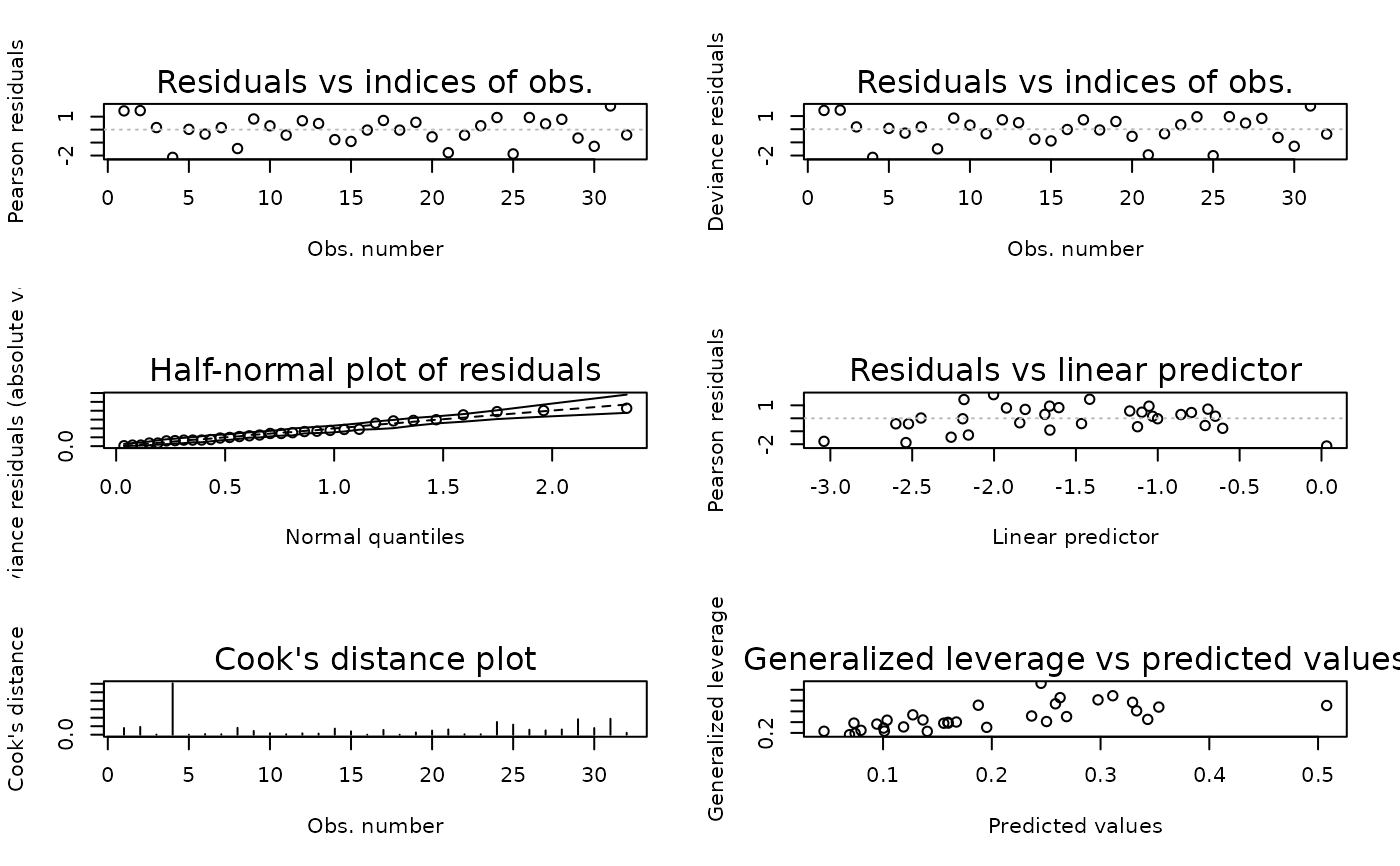
## Figure 2
par(mfrow = c(3, 2))
plot(gy2, which = 1, type = "pearson", sub.caption = "")
plot(gy2, which = 1, type = "deviance", sub.caption = "")
plot(gy2, which = 5, type = "deviance", sub.caption = "")
plot(gy2, which = 4, type = "pearson", sub.caption = "")
plot(gy2, which = 2:3)
 par(mfrow = c(1, 1))
## exclude 4th observation
gy2a <- update(gy2, subset = -4)
gy2a
#>
#> Call:
#> betareg(formula = yield ~ batch + temp, data = GasolineYield, subset = -4)
#>
#> Coefficients (mean model with logit link):
#> (Intercept) batch1 batch2 batch3 batch4 batch5
#> -6.35647 1.88688 1.37039 1.62512 1.08066 1.15158
#> batch6 batch7 batch8 batch9 temp
#> 1.05766 0.56522 0.50066 0.38523 0.01146
#>
#> Phi coefficients (precision model with identity link):
#> (phi)
#> 577.8
#>
summary(gy2a)
#>
#> Call:
#> betareg(formula = yield ~ batch + temp, data = GasolineYield, subset = -4)
#>
#> Quantile residuals:
#> Min 1Q Median 3Q Max
#> -2.0153 -0.8176 0.0897 0.6948 2.0746
#>
#> Coefficients (mean model with logit link):
#> Estimate Std. Error z value Pr(>|z|)
#> (Intercept) -6.3564713 0.1716020 -37.042 < 2e-16 ***
#> batch1 1.8868782 0.1001837 18.834 < 2e-16 ***
#> batch2 1.3703911 0.1042352 13.147 < 2e-16 ***
#> batch3 1.6251199 0.1028326 15.804 < 2e-16 ***
#> batch4 1.0806596 0.0897855 12.036 < 2e-16 ***
#> batch5 1.1515826 0.0906857 12.699 < 2e-16 ***
#> batch6 1.0576556 0.0929172 11.383 < 2e-16 ***
#> batch7 0.5652219 0.0956100 5.912 3.39e-09 ***
#> batch8 0.5006625 0.0953210 5.252 1.50e-07 ***
#> batch9 0.3852258 0.1037500 3.713 0.000205 ***
#> temp 0.0114588 0.0003945 29.050 < 2e-16 ***
#>
#> Phi coefficients (precision model with identity link):
#> Estimate Std. Error z value Pr(>|z|)
#> (phi) 577.8 146.7 3.938 8.22e-05 ***
#> ---
#> Signif. codes: 0 '***' 0.001 '**' 0.01 '*' 0.05 '.' 0.1 ' ' 1
#>
#> Type of estimator: ML (maximum likelihood)
#> Log-likelihood: 86.62 on 12 Df
#> Pseudo R-squared: 0.9662
#> Number of iterations: 51 (BFGS) + 4 (Fisher scoring)
## IGNORE_RDIFF_END
par(mfrow = c(1, 1))
## exclude 4th observation
gy2a <- update(gy2, subset = -4)
gy2a
#>
#> Call:
#> betareg(formula = yield ~ batch + temp, data = GasolineYield, subset = -4)
#>
#> Coefficients (mean model with logit link):
#> (Intercept) batch1 batch2 batch3 batch4 batch5
#> -6.35647 1.88688 1.37039 1.62512 1.08066 1.15158
#> batch6 batch7 batch8 batch9 temp
#> 1.05766 0.56522 0.50066 0.38523 0.01146
#>
#> Phi coefficients (precision model with identity link):
#> (phi)
#> 577.8
#>
summary(gy2a)
#>
#> Call:
#> betareg(formula = yield ~ batch + temp, data = GasolineYield, subset = -4)
#>
#> Quantile residuals:
#> Min 1Q Median 3Q Max
#> -2.0153 -0.8176 0.0897 0.6948 2.0746
#>
#> Coefficients (mean model with logit link):
#> Estimate Std. Error z value Pr(>|z|)
#> (Intercept) -6.3564713 0.1716020 -37.042 < 2e-16 ***
#> batch1 1.8868782 0.1001837 18.834 < 2e-16 ***
#> batch2 1.3703911 0.1042352 13.147 < 2e-16 ***
#> batch3 1.6251199 0.1028326 15.804 < 2e-16 ***
#> batch4 1.0806596 0.0897855 12.036 < 2e-16 ***
#> batch5 1.1515826 0.0906857 12.699 < 2e-16 ***
#> batch6 1.0576556 0.0929172 11.383 < 2e-16 ***
#> batch7 0.5652219 0.0956100 5.912 3.39e-09 ***
#> batch8 0.5006625 0.0953210 5.252 1.50e-07 ***
#> batch9 0.3852258 0.1037500 3.713 0.000205 ***
#> temp 0.0114588 0.0003945 29.050 < 2e-16 ***
#>
#> Phi coefficients (precision model with identity link):
#> Estimate Std. Error z value Pr(>|z|)
#> (phi) 577.8 146.7 3.938 8.22e-05 ***
#> ---
#> Signif. codes: 0 '***' 0.001 '**' 0.01 '*' 0.05 '.' 0.1 ' ' 1
#>
#> Type of estimator: ML (maximum likelihood)
#> Log-likelihood: 86.62 on 12 Df
#> Pseudo R-squared: 0.9662
#> Number of iterations: 51 (BFGS) + 4 (Fisher scoring)
## IGNORE_RDIFF_END