(No) Myopic Loss Aversion in Adolescents
LossAversion.RdData from a behavioral economics experiment assessing the extent of myopic loss aversion among adolescents (mostly aged 11 to 19).
Usage
data("LossAversion", package = "betareg")Format
A data frame containing 570 observations on 7 variables.
- invest
numeric. Average proportion of tokens invested across all 9 rounds.
- gender
factor. Gender of the player (or team of players).
- male
factor. Was (at least one of) the player(s) male (in the team)?
- age
numeric. Age in years (averaged for teams).
- treatment
factor. Type of treatment: long vs. short.
- grade
factor. School grades: 6-8 (11-14 years) vs. 10-12 (15-18 years).
- arrangement
factor. Is the player a single player or team of two?
Details
Myopic loss aversion is a phenomenon in behavioral economics, where individuals do not behave economically rationally when making short-term decisions under uncertainty. Example: In lotteries with positive expected payouts investments are lower than the maximum possible (loss aversion). This effect is enhanced for short-term investments (myopia or short-sightedness).
The data in LossAversion were collected by Matthias Sutter and
Daniela Glätzle-Rützler (Universität Innsbruck) in an experiment with
high-school students in Tyrol, Austria (Schwaz and Innsbruck). The students
could invest X tokens (0-100) in each of 9 rounds in a lottery. The payouts
were 100 + 2.5 * X tokens with probability 1/3 and 100 - X tokens with
probability 2/3. Thus, the expected payouts were 100 + 1/6 * X tokens.
Depending on the treatment in the experiment, the investments could either be
modified in each round (treatment: "short") or only in round 1, 4, 7
(treatment "long"). Decisions were either made alone or in teams of two. The
tokens were converted to monetary payouts using a conversion of
EUR 0.5 per 100 tokens for lower grades (Unterstufe, 6-8) or EUR 1.0 per 100
tokens for upper grades (Oberstufe, 10-12).
From the myopic loss aversion literature (on adults) one would expect that the investments of the players (either single players or teams of two) would depend on all factors: Investments should be
lower in the short treatment (which would indicate myopia),
higher for teams (indicating a reduction in loss aversion),
higher for (teams with) male players,
increase with age/grade.
See Glätzle-Rützler et al. (2015) for more details and references to the literature. In their original analysis, the investments are analyzes using a panel structure (i.e., 9 separate investments for each team). Here, the data are averaged across rounds for each player, leading to qualitatively similar results. The full data along with replication materials are available in the Harvard Dataverse.
Kosmidis and Zeileis (2026) revisit the data using extended-support beta mixture (XBX) regression, which can simultaneously capture both the probability of rational behavior and the mean amount of loss aversion.
Source
Glätzle-Rützler D, Sutter M, Zeileis A (2020). Replication Data for: No Myopic Loss Aversion in Adolescents? - An Experimental Note. Harvard Dataverse, UNF:6:6hVtbHavJAFYfL7dDl7jqA==. doi:10.7910/DVN/IHFZAK
References
Glätzle-Rützler D, Sutter M, Zeileis A (2015). No Myopic Loss Aversion in Adolescents? – An Experimental Note. Journal of Economic Behavior & Organization, 111, 169–176. doi:10.1016/j.jebo.2014.12.021
Kosmidis I, Zeileis A (2026). Extended-Support Beta Regression for [0, 1] Responses. Journal of the Royal Statistical Society C, 75(1), 139–157. doi:10.1093/jrsssc/qlaf039
Examples
options(digits = 4)
## data and add ad-hoc scaling (a la Smithson & Verkuilen)
data("LossAversion", package = "betareg")
LossAversion <- transform(LossAversion,
invests = (invest * (nrow(LossAversion) - 1) + 0.5)/nrow(LossAversion))
## models: normal (with constant variance), beta, extended-support beta mixture
la_n <- lm(invest ~ grade * (arrangement + age) + male, data = LossAversion)
summary(la_n)
#>
#> Call:
#> lm(formula = invest ~ grade * (arrangement + age) + male, data = LossAversion)
#>
#> Residuals:
#> Min 1Q Median 3Q Max
#> -0.7735 -0.1967 0.0024 0.1916 0.5724
#>
#> Coefficients:
#> Estimate Std. Error t value Pr(>|t|)
#> (Intercept) 0.2844 0.1575 1.81 0.07136 .
#> grade10-12 -0.8437 0.2815 -3.00 0.00284 **
#> arrangementteam 0.0628 0.0302 2.08 0.03788 *
#> age 0.0115 0.0124 0.93 0.35041
#> maleyes 0.1035 0.0232 4.46 9.9e-06 ***
#> grade10-12:arrangementteam 0.1507 0.0455 3.32 0.00097 ***
#> grade10-12:age 0.0458 0.0185 2.47 0.01380 *
#> ---
#> Signif. codes: 0 ‘***’ 0.001 ‘**’ 0.01 ‘*’ 0.05 ‘.’ 0.1 ‘ ’ 1
#>
#> Residual standard error: 0.247 on 563 degrees of freedom
#> Multiple R-squared: 0.158, Adjusted R-squared: 0.149
#> F-statistic: 17.7 on 6 and 563 DF, p-value: <2e-16
#>
# \donttest{
la_b <- betareg(invests ~ grade * (arrangement + age) + male | arrangement + male + grade,
data = LossAversion)
summary(la_b)
#>
#> Call:
#> betareg(formula = invests ~ grade * (arrangement + age) + male | arrangement +
#> male + grade, data = LossAversion)
#>
#> Quantile residuals:
#> Min 1Q Median 3Q Max
#> -3.948 -0.594 -0.042 0.554 4.439
#>
#> Coefficients (mean model with logit link):
#> Estimate Std. Error z value Pr(>|z|)
#> (Intercept) -1.4139 0.6197 -2.28 0.0225 *
#> grade10-12 -2.9435 1.2520 -2.35 0.0187 *
#> arrangementteam 0.2250 0.1175 1.92 0.0554 .
#> age 0.0906 0.0486 1.87 0.0621 .
#> maleyes 0.4553 0.0990 4.60 4.2e-06 ***
#> grade10-12:arrangementteam 0.6549 0.2003 3.27 0.0011 **
#> grade10-12:age 0.1513 0.0806 1.88 0.0605 .
#>
#> Phi coefficients (precision model with log link):
#> Estimate Std. Error z value Pr(>|z|)
#> (Intercept) 1.194 0.084 14.21 < 2e-16 ***
#> arrangementteam 0.406 0.122 3.33 0.00087 ***
#> maleyes -0.555 0.113 -4.93 8.2e-07 ***
#> grade10-12 -0.553 0.104 -5.31 1.1e-07 ***
#> ---
#> Signif. codes: 0 '***' 0.001 '**' 0.01 '*' 0.05 '.' 0.1 ' ' 1
#>
#> Type of estimator: ML (maximum likelihood)
#> Log-likelihood: 94.4 on 11 Df
#> Pseudo R-squared: 0.154
#> Number of iterations: 24 (BFGS) + 3 (Fisher scoring)
la_xbx <- betareg(invest ~ grade * (arrangement + age) + male | arrangement + male + grade,
data = LossAversion)
#> Loading required namespace: numDeriv
summary(la_xbx)
#>
#> Call:
#> betareg(formula = invest ~ grade * (arrangement + age) + male | arrangement +
#> male + grade, data = LossAversion)
#>
#> Randomized quantile residuals:
#> Min 1Q Median 3Q Max
#> -3.236 -0.693 -0.015 0.698 3.768
#>
#> Coefficients (mu model with logit link):
#> Estimate Std. Error z value Pr(>|z|)
#> (Intercept) -0.8650 0.5193 -1.67 0.09577 .
#> grade10-12 -3.0962 1.0529 -2.94 0.00328 **
#> arrangementteam 0.2079 0.0987 2.11 0.03508 *
#> age 0.0489 0.0406 1.20 0.22857
#> maleyes 0.3792 0.0842 4.50 6.6e-06 ***
#> grade10-12:arrangementteam 0.5672 0.1690 3.36 0.00079 ***
#> grade10-12:age 0.1687 0.0677 2.49 0.01275 *
#>
#> Phi coefficients (phi model with log link):
#> Estimate Std. Error z value Pr(>|z|)
#> (Intercept) 1.756 0.128 13.70 < 2e-16 ***
#> arrangementteam 0.325 0.145 2.25 0.02446 *
#> maleyes -0.484 0.136 -3.56 0.00037 ***
#> grade10-12 -0.316 0.131 -2.41 0.01608 *
#>
#> Exceedence parameter (extended-support xbetax model):
#> Estimate Std. Error z value Pr(>|z|)
#> Log(nu) -2.273 0.245 -9.27 <2e-16 ***
#> ---
#> Signif. codes: 0 '***' 0.001 '**' 0.01 '*' 0.05 '.' 0.1 ' ' 1
#>
#> Exceedence parameter nu: 0.103
#> Type of estimator: ML (maximum likelihood)
#> Log-likelihood: -71.8 on 12 Df
#> Number of iterations in BFGS optimization: 45
## coefficients in XBX are typically somewhat shrunken compared to beta
cbind(XBX = coef(la_xbx), Beta = c(coef(la_b), NA))
#> XBX Beta
#> (Intercept) -0.86495 -1.41389
#> grade10-12 -3.09624 -2.94347
#> arrangementteam 0.20790 0.22498
#> age 0.04889 0.09061
#> maleyes 0.37925 0.45534
#> grade10-12:arrangementteam 0.56724 0.65487
#> grade10-12:age 0.16866 0.15129
#> (phi)_(Intercept) 1.75629 1.19429
#> (phi)_arrangementteam 0.32525 0.40631
#> (phi)_maleyes -0.48406 -0.55481
#> (phi)_grade10-12 -0.31593 -0.55271
#> Log(nu) -2.27289 NA
## predictions on subset: (at least one) male players, higher grades, around age 16
la <- subset(LossAversion, male == "yes" & grade == "10-12" & age >= 15 & age <= 17)
la_nd <- data.frame(arrangement = c("single", "team"), male = "yes", age = 16, grade = "10-12")
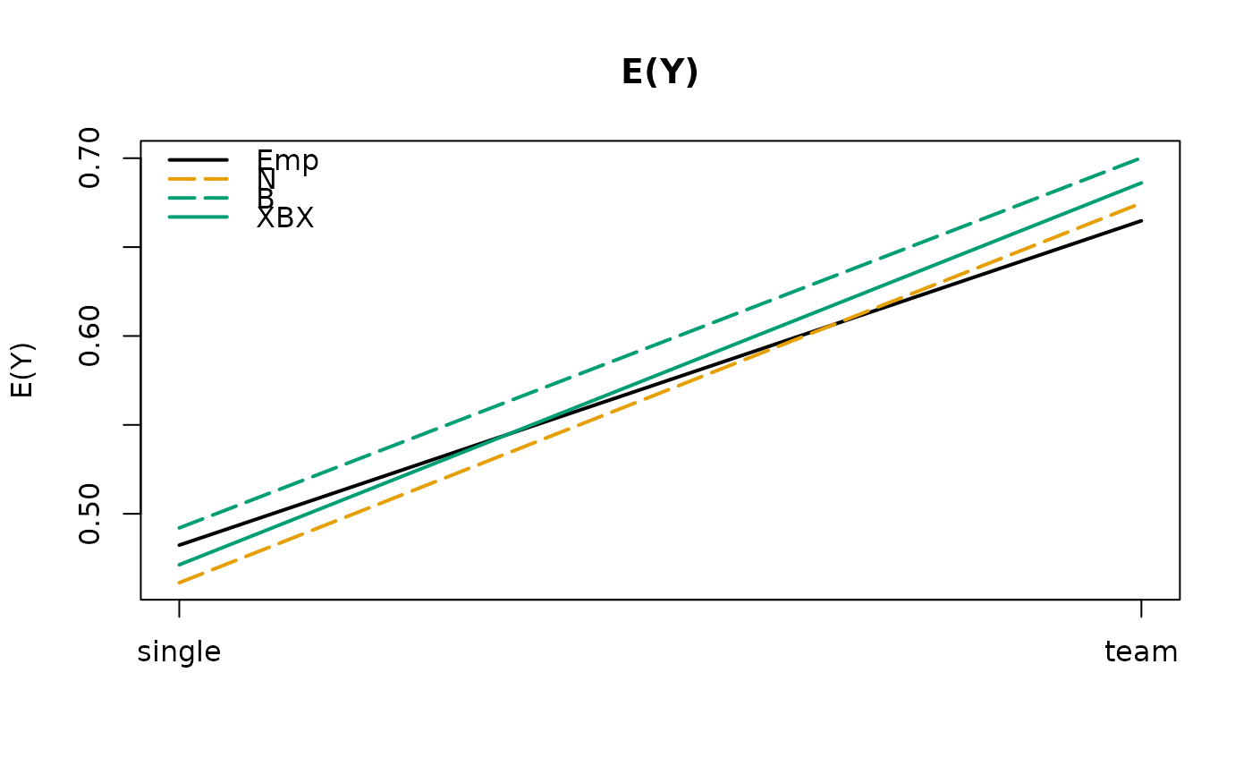
## empirical vs fitted E(Y)
la_nd$mean_emp <- aggregate(invest ~ arrangement, data = la, FUN = mean)$invest
la_nd$mean_n <- predict(la_n, la_nd)
la_nd$mean_b <- predict(la_b, la_nd)
la_nd$mean_xbx <- predict(la_xbx, la_nd)
la_nd
#> arrangement male age grade mean_emp mean_n mean_b mean_xbx
#> 1 single yes 16 10-12 0.4824 0.4612 0.4921 0.4713
#> 2 team yes 16 10-12 0.6648 0.6747 0.7002 0.6861
## visualization: all means rather similar
la_mod <- c("Emp", "N", "B", "XBX")
la_col <- unname(palette.colors())[c(1, 2, 4, 4)]
la_lty <- c(1, 5, 5, 1)
matplot(la_nd[, paste0("mean_", tolower(la_mod))], type = "l",
col = la_col, lty = la_lty, lwd = 2, ylab = "E(Y)", main = "E(Y)", xaxt = "n")
axis(1, at = 1:2, labels = la_nd$arrangement)
legend("topleft", la_mod, col = la_col, lty = la_lty, lwd = 2, bty = "n")
 ## empirical vs. fitted P(Y > 0.95)
la_nd$prob_emp <- aggregate(invest >= 0.95 ~ arrangement, data = la, FUN = mean)$invest
la_nd$prob_n <- pnorm(0.95, mean = la_nd$mean_n, sd = summary(la_n)$sigma, lower.tail = FALSE)
la_nd$prob_b <- 1 - predict(la_b, la_nd, type = "probability", at = 0.95)
la_nd$prob_xbx <- 1 - predict(la_xbx, la_nd, type = "probability", at = 0.95)
la_nd[, -(5:8)]
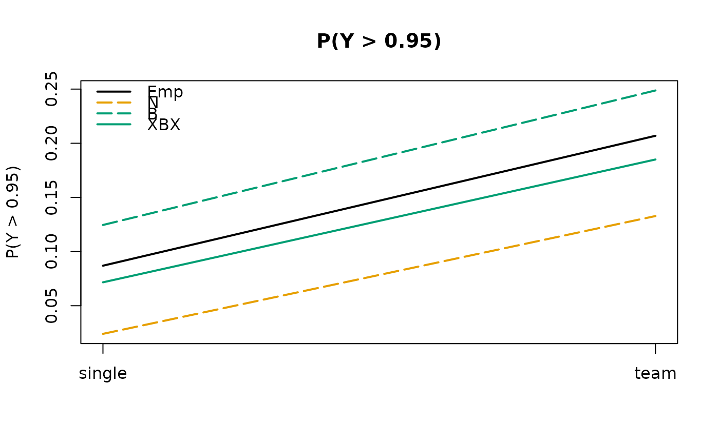
#> arrangement male age grade prob_emp prob_n prob_b prob_xbx
#> 1 single yes 16 10-12 0.08696 0.02403 0.1245 0.07161
#> 2 team yes 16 10-12 0.20690 0.13280 0.2487 0.18501
## visualization: only XBX works well
matplot(la_nd[, paste0("prob_", tolower(la_mod))], type = "l",
col = la_col, lty = la_lty, lwd = 2, ylab = "P(Y > 0.95)", main = "P(Y > 0.95)", xaxt = "n")
axis(1, at = 1:2, labels = la_nd$arrangement)
legend("topleft", la_mod, col = la_col, lty = la_lty, lwd = 2, bty = "n")
## empirical vs. fitted P(Y > 0.95)
la_nd$prob_emp <- aggregate(invest >= 0.95 ~ arrangement, data = la, FUN = mean)$invest
la_nd$prob_n <- pnorm(0.95, mean = la_nd$mean_n, sd = summary(la_n)$sigma, lower.tail = FALSE)
la_nd$prob_b <- 1 - predict(la_b, la_nd, type = "probability", at = 0.95)
la_nd$prob_xbx <- 1 - predict(la_xbx, la_nd, type = "probability", at = 0.95)
la_nd[, -(5:8)]
#> arrangement male age grade prob_emp prob_n prob_b prob_xbx
#> 1 single yes 16 10-12 0.08696 0.02403 0.1245 0.07161
#> 2 team yes 16 10-12 0.20690 0.13280 0.2487 0.18501
## visualization: only XBX works well
matplot(la_nd[, paste0("prob_", tolower(la_mod))], type = "l",
col = la_col, lty = la_lty, lwd = 2, ylab = "P(Y > 0.95)", main = "P(Y > 0.95)", xaxt = "n")
axis(1, at = 1:2, labels = la_nd$arrangement)
legend("topleft", la_mod, col = la_col, lty = la_lty, lwd = 2, bty = "n")
 # }
# }