Create an Extended-Support Beta Mixture Distribution

Class and methods for extended-support beta distributions using the workflow from the distributions3 package.

Usage

XBetaX(mu = numeric(), phi = numeric(), nu = NULL)

Arguments

mu: numeric. The mean of the underlying beta distribution on [-nu, 1 + nu].
phi: numeric. The precision parameter of the underlying beta distribution on [-nu, 1 + nu].
nu: numeric. Mean of the exponentially-distributed exceedence parameter for the underlying beta distribution on [-nu, 1 + nu] that is censored to [0, 1]. By default nu = 0 is used.

Details

The extended-support beta mixture distribution is a continuous mixture of extended-support beta distributions on [0, 1] where the underlying exceedence parameter is exponentially distributed with mean nu. Thus, if nu > 0, the resulting distribution has point masses on the boundaries 0 and 1 with larger values of nu leading to higher boundary probabilities. For nu = 0 (the default), the distribution reduces to the classic beta distribution (in regression parameterization) without boundary observations.

Value

A XBetaX distribution object.

Examples

## package and random seed
library("distributions3")
set.seed(6020)

## three beta distributions
X <- XBetaX(
  mu  = c(0.25, 0.50, 0.75),
  phi = c(1, 1, 2),
  nu = c(0, 0.1, 0.2)
)
# \donttest{
X
#> [1] "XBetaX(mu = 0.25, phi = 1, nu = 0.0)"
#> [2] "XBetaX(mu = 0.50, phi = 1, nu = 0.1)"
#> [3] "XBetaX(mu = 0.75, phi = 2, nu = 0.2)"

## compute moments of the distribution
mean(X)
#> [1] 0.2500 0.5000 0.7813
variance(X)
#> [1] 0.09375 0.14933 0.08290

## support interval (minimum and maximum)
support(X)
#>      min max
#> [1,]   0   1
#> [2,]   0   1
#> [3,]   0   1

## it is only continuous when there are no point masses on the boundary
is_continuous(X)
#> [1]  TRUE FALSE FALSE
cdf(X, 0)
#> [1] 0.0000 0.1613 0.0223
cdf(X, 1, lower.tail = FALSE)
#> [1] 0.0000 0.1613 0.4004

## simulate random variables
random(X, 5)
#>          r_1     r_2      r_3    r_4     r_5
#> [1,] 0.01770 0.03197 0.009185 0.3511 0.03418
#> [2,] 0.03065 0.00000 0.159693 0.4697 0.62766
#> [3,] 0.40195 1.00000 0.675082 0.9256 1.00000

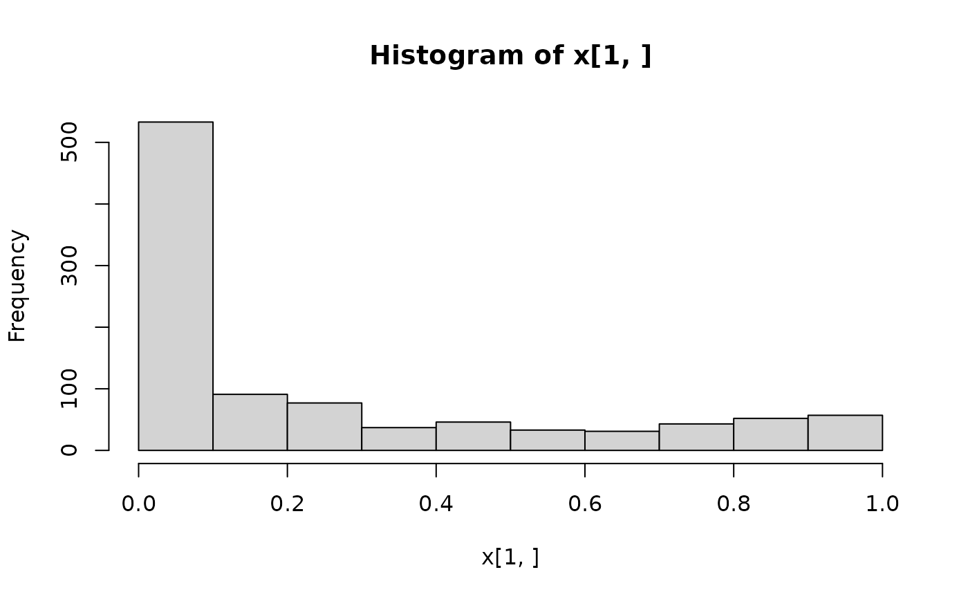
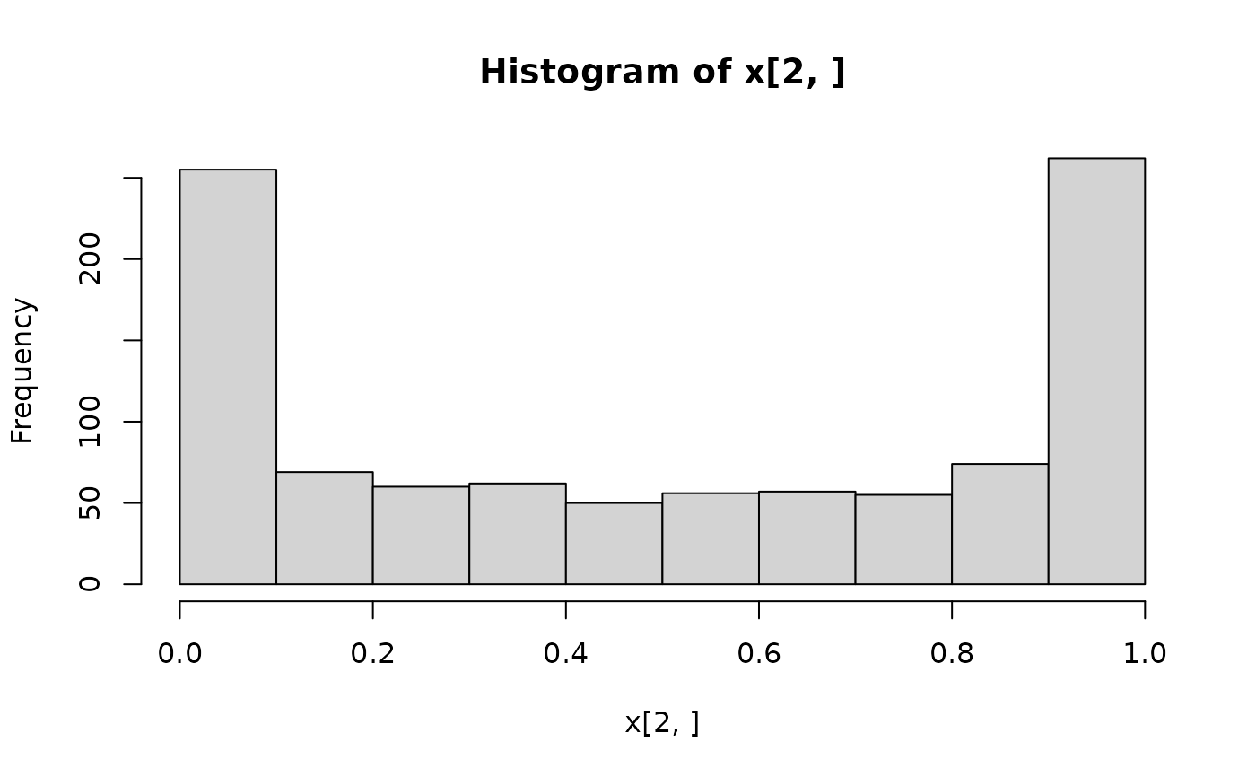
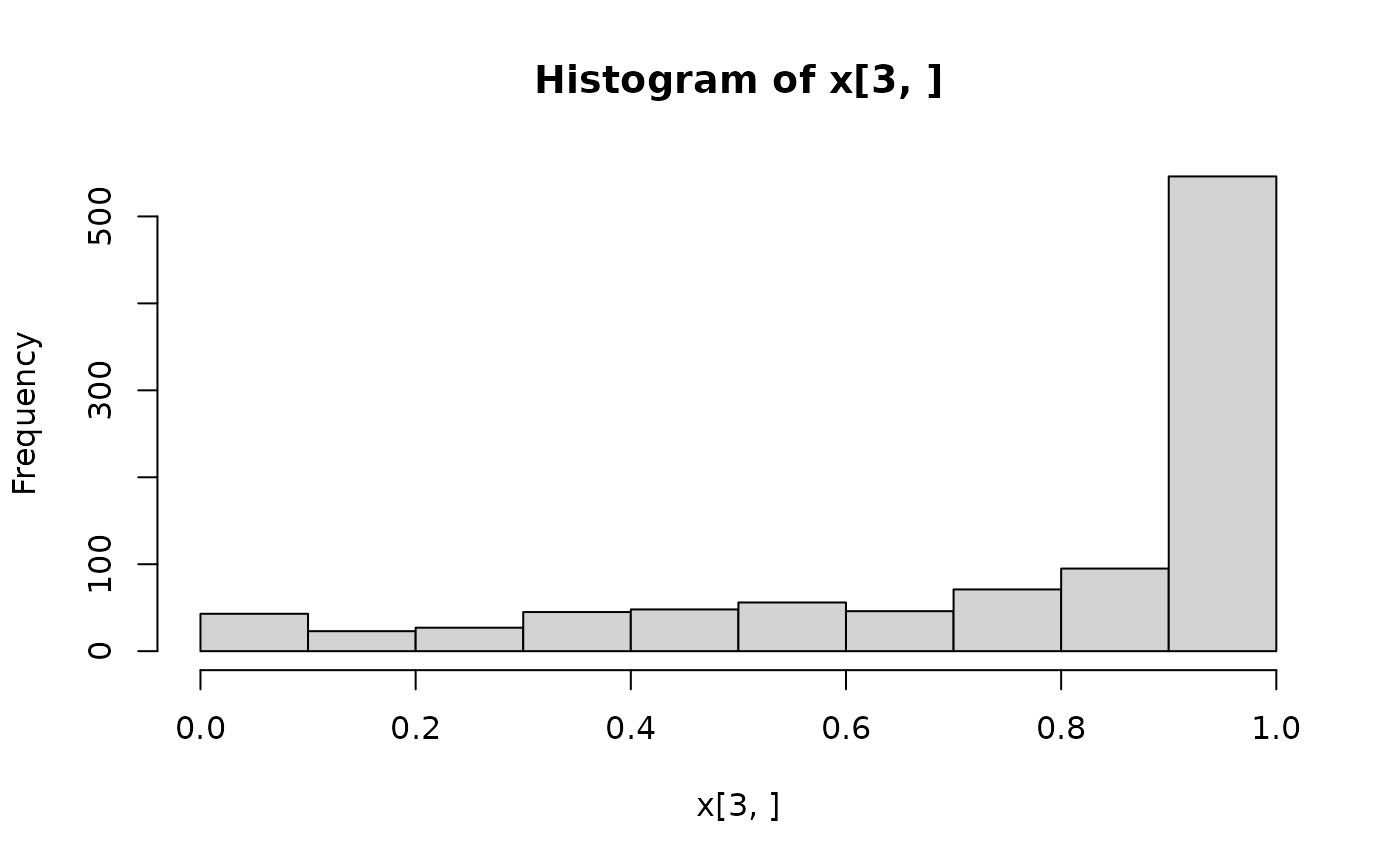
## histograms of 1,000 simulated observations
x <- random(X, 1000)
hist(x[1, ])

hist(x[2, ])

hist(x[3, ])


## probability density function (PDF) and log-density (or log-likelihood)
x <- c(0.25, 0.5, 0.75)
pdf(X, x)
#> [1] 0.6841 0.5425 0.7406
pdf(X, x, log = TRUE)
#> [1] -0.3797 -0.6116 -0.3004
log_pdf(X, x)
#> [1] -0.3797 -0.6116 -0.3004

## cumulative distribution function (CDF)
cdf(X, x)
#> [1] 0.6454 0.5000 0.3312

## quantiles
quantile(X, 0.5)
#> [1] 0.09331 0.50000 0.93231

## cdf() and quantile() are inverses (except at censoring points)
cdf(X, quantile(X, 0.5))
#> [1] 0.5 0.5 0.5
quantile(X, cdf(X, 1))
#> [1] 1 1 1

## all methods above can either be applied elementwise or for
## all combinations of X and x, if length(X) = length(x),
## also the result can be assured to be a matrix via drop = FALSE
p <- c(0.05, 0.5, 0.95)
quantile(X, p, elementwise = FALSE)
#>         q_0.05   q_0.5 q_0.95
#> [1,] 9.513e-06 0.09331 0.9118
#> [2,] 0.000e+00 0.50000 1.0000
#> [3,] 1.354e-01 0.93231 1.0000
quantile(X, p, elementwise = TRUE)
#> [1] 9.513e-06 5.000e-01 1.000e+00
quantile(X, p, elementwise = TRUE, drop = FALSE)
#>       quantile
#> [1,] 9.513e-06
#> [2,] 5.000e-01
#> [3,] 1.000e+00

## compare theoretical and empirical mean from 1,000 simulated observations
cbind(
  "theoretical" = mean(X),
  "empirical" = rowMeans(random(X, 1000))
)
#>      theoretical empirical
#> [1,]      0.2500    0.2403
#> [2,]      0.5000    0.4936
#> [3,]      0.7813    0.7936
# }