Family Objects for (Extended-Support) Beta Regression
betar_family.RdFamily objects for distributional regression with the (extended-support) beta distribution via bamlss or gamlss2.
Usage
betar_family(link = "logit", link.phi = "log", ...)

xbetax_family(link = "logit", link.phi = "log", link.nu = "log",
  quad = 20, tol = .Machine$double.eps^0.7, ...)
Arguments
- link
character specification of the link function in the mean model (mu). Currently,
"logit","probit","cloglog","cauchit","log","loglog"are supported.- link.phi
character specification of the link function in the precision model (phi). Currently,
"log","identity","sqrt"are supported.- link.nu
character specification of the link function in the exceedence model (nu). Currently,
"log","identity","sqrt"are supported.- quad
numeric. The number of quadrature points for numeric integration of the continuous mixture in
dxbetax. Alternatively, a matrix with nodes and weights for the quadrature points can be specified.- tol
numeric. Accuracy (convergence tolerance) for numerically determining quantiles based on
unirootandpxbetax.- ...
Arguments passed to functions that are called within the family object.
Details
Family objects for bamlss (Umlauf et al. 2019, 2021) and gamlss2
(Umlauf et al. 2025) are essentially lists of functions providing a standardized
interface to the d/p/q/r functions of distributions. Hence, betar_family
interfaces the classical beta distribution in regression specification, see
dbetar. Analogously, xbetax_family interfaces the
extended-support beta mixture specification (Kosmidis and Zeileis 2026),
see dxbetax.
Value
A list of class family.bamlss.
References
Kosmidis I, Zeileis A (2026). Extended-Support Beta Regression for [0, 1] Responses. Journal of the Royal Statistical Society C, 75(1), 139–157. doi:10.1093/jrsssc/qlaf039
Umlauf N, Klein N, Zeileis A (2019). BAMLSS: Bayesian Additive Models for Location, Scale and Shape (and Beyond). Journal of Computational and Graphical Statistics, 27(3), 612–627. doi:10.1080/10618600.2017.1407325
Umlauf N, Klein N, Simon T, Zeileis A (2021). bamlss: A Lego Toolbox for Flexible Bayesian Regression (and Beyond). Journal of Statistical Software, 100(4), 1–53. doi:10.18637/jss.v100.i04
Umlauf N, Stasinopoulos M, Rigby R, Stauffer R (2025). gamlss2: Infrastructure for Flexible Distributional Regression. R package version 0.1-0. https://gamlss-dev.github.io/gamlss2/
Examples
## IGNORE_RDIFF_BEGIN
#> Loading required namespace: bamlss
## package and data
library("betareg")
library("bamlss")
#> Loading required package: coda
#> Loading required package: colorspace
#> Loading required package: mgcv
#> Loading required package: nlme
#> This is mgcv 1.9-4. For overview type '?mgcv'.
#> -
#> For citation info, use citation("bamlss") and see http://www.bamlss.org/.
#>
#> Attaching package: ‘bamlss’
#> The following object is masked from ‘package:mgcv’:
#>
#> smooth.construct
#> The following object is masked from ‘package:flexmix’:
#>
#> parameters
data("ReadingSkills", package = "betareg")
## classical beta regression via ML
rs1 <- betareg(accuracy ~ dyslexia * iq | dyslexia + iq, data = ReadingSkills)
## Bayesian additive model (with low number of iterations to speed up the example)
set.seed(0)
rs2 <- bamlss(accuracy ~ s(iq, by = dyslexia) | dyslexia + iq, data = ReadingSkills,
family = betar_family(), eps = 1e-7, n.iter = 400, burnin = 100)
#> AICc -0.8829 logPost -64.6792 logLik 21.6241 edf 13.973 eps 1.0000 iteration 1
#> AICc -51.8915 logPost -25.8044 logLik 39.7035 edf 10.242 eps 2.8731 iteration 2
#> AICc -68.1251 logPost -7.3858 logLik 46.8183 edf 9.6642 eps 0.5561 iteration 3
#> AICc -73.1290 logPost 4.7269 logLik 48.3399 edf 9.0783 eps 0.0895 iteration 4
#> AICc -74.7842 logPost 5.5545 logLik 49.1675 edf 9.0783 eps 0.0629 iteration 5
#> AICc -75.7464 logPost 6.0357 logLik 49.6487 edf 9.0783 eps 0.0559 iteration 6
#> AICc -76.3072 logPost 6.3160 logLik 49.9291 edf 9.0783 eps 0.2490 iteration 7
#> AICc -77.3399 logPost 6.8324 logLik 50.4454 edf 9.0783 eps 0.2694 iteration 8
#> AICc -77.6557 logPost 6.9903 logLik 50.6033 edf 9.0783 eps 0.0207 iteration 9
#> AICc -77.8176 logPost 7.0713 logLik 50.6843 edf 9.0783 eps 0.0123 iteration 10
#> AICc -80.2391 logPost 8.7295 logLik 50.7321 edf 8.3559 eps 0.0099 iteration 11
#> AICc -81.1323 logPost -61.6299 logLik 50.7922 edf 8.1090 eps 0.0333 iteration 12
#> AICc -81.3164 logPost -654.389 logLik 50.8351 edf 8.0774 eps 0.0089 iteration 13
#> AICc -81.3726 logPost -4694.96 logLik 50.8579 edf 8.0740 eps 0.0054 iteration 14
#> AICc -81.4322 logPost -25766.3 logLik 50.8816 edf 8.0700 eps 0.0077 iteration 15
#> AICc -81.6598 logPost -2043.53 logLik 50.9498 edf 8.0406 eps 0.0179 iteration 16
#> AICc -82.3830 logPost -8852.97 logLik 51.1594 edf 7.9421 eps 0.0137 iteration 17
#> AICc -82.7904 logPost -13085.5 logLik 51.2898 edf 7.8944 eps 0.0124 iteration 18
#> AICc -82.9776 logPost -13740.2 logLik 51.3740 edf 7.8883 eps 0.0431 iteration 19
#> AICc -83.0956 logPost -13809.0 logLik 51.4431 edf 7.8949 eps 0.0096 iteration 20
#> AICc -83.2026 logPost -13815.6 logLik 51.4812 edf 7.8848 eps 0.0058 iteration 21
#> AICc -83.2582 logPost -13816.0 logLik 51.5109 edf 7.8861 eps 0.0574 iteration 22
#> AICc -83.3488 logPost -13815.9 logLik 51.5729 edf 7.8970 eps 0.0084 iteration 23
#> AICc -83.4298 logPost -13815.7 logLik 51.5929 edf 7.8836 eps 0.0035 iteration 24
#> AICc -83.4578 logPost -13815.6 logLik 51.6069 edf 7.8837 eps 0.0029 iteration 25
#> AICc -83.4771 logPost -13815.4 logLik 51.6166 edf 7.8837 eps 0.0025 iteration 26
#> AICc -83.4921 logPost -13815.3 logLik 51.6242 edf 7.8837 eps 0.0042 iteration 27
#> AICc -83.5087 logPost -13815.3 logLik 51.6291 edf 7.8815 eps 0.0021 iteration 28
#> AICc -83.5136 logPost -13815.2 logLik 51.6323 edf 7.8820 eps 0.0016 iteration 29
#> AICc -83.5176 logPost -13815.1 logLik 51.6343 edf 7.8820 eps 0.0013 iteration 30
#> AICc -83.5199 logPost -13815.1 logLik 51.6355 edf 7.8820 eps 0.0011 iteration 31
#> AICc -83.5219 logPost -13815.1 logLik 51.6365 edf 7.8820 eps 0.0042 iteration 32
#> AICc -83.5216 logPost -13815.0 logLik 51.6382 edf 7.8832 eps 0.0022 iteration 33
#> AICc -83.5300 logPost -13815.0 logLik 51.6383 edf 7.8806 eps 0.0009 iteration 34
#> AICc -83.5294 logPost -13815.0 logLik 51.6384 edf 7.8808 eps 0.0003 iteration 35
#> AICc -83.5293 logPost -13815.0 logLik 51.6384 edf 7.8809 eps 0.0000 iteration 36
#> AICc -83.5293 logPost -13815.0 logLik 51.6384 edf 7.8809 eps 0.0000 iteration 37
#> AICc -83.5293 logPost -13815.0 logLik 51.6384 edf 7.8809 eps 0.0000 iteration 38
#> AICc -83.5293 logPost -13815.0 logLik 51.6384 edf 7.8809 eps 0.0000 iteration 39
#> AICc -83.5293 logPost -13815.0 logLik 51.6384 edf 7.8809 eps 0.0000 iteration 39
#> elapsed time: 2.67sec
#> Starting the sampler...
#>
#> | | 0% 2.18sec
#> |* | 5% 2.36sec 0.12sec
#> |** | 10% 2.11sec 0.23sec
#> |*** | 15% 1.89sec 0.33sec
#> |**** | 20% 1.76sec 0.44sec
#> |***** | 25% 1.65sec 0.55sec
#> |****** | 30% 1.55sec 0.66sec
#> |******* | 35% 1.46sec 0.78sec
#> |******** | 40% 1.38sec 0.92sec
#> |********* | 45% 1.27sec 1.04sec
#> |********** | 50% 1.15sec 1.15sec
#> |*********** | 55% 1.03sec 1.26sec
#> |************ | 60% 0.92sec 1.38sec
#> |************* | 65% 0.80sec 1.49sec
#> |************** | 70% 0.69sec 1.61sec
#> |*************** | 75% 0.57sec 1.72sec
#> |**************** | 80% 0.47sec 1.87sec
#> |***************** | 85% 0.35sec 1.99sec
#> |****************** | 90% 0.23sec 2.11sec
#> |******************* | 95% 0.12sec 2.23sec
#> |********************| 100% 0.00sec 2.34sec
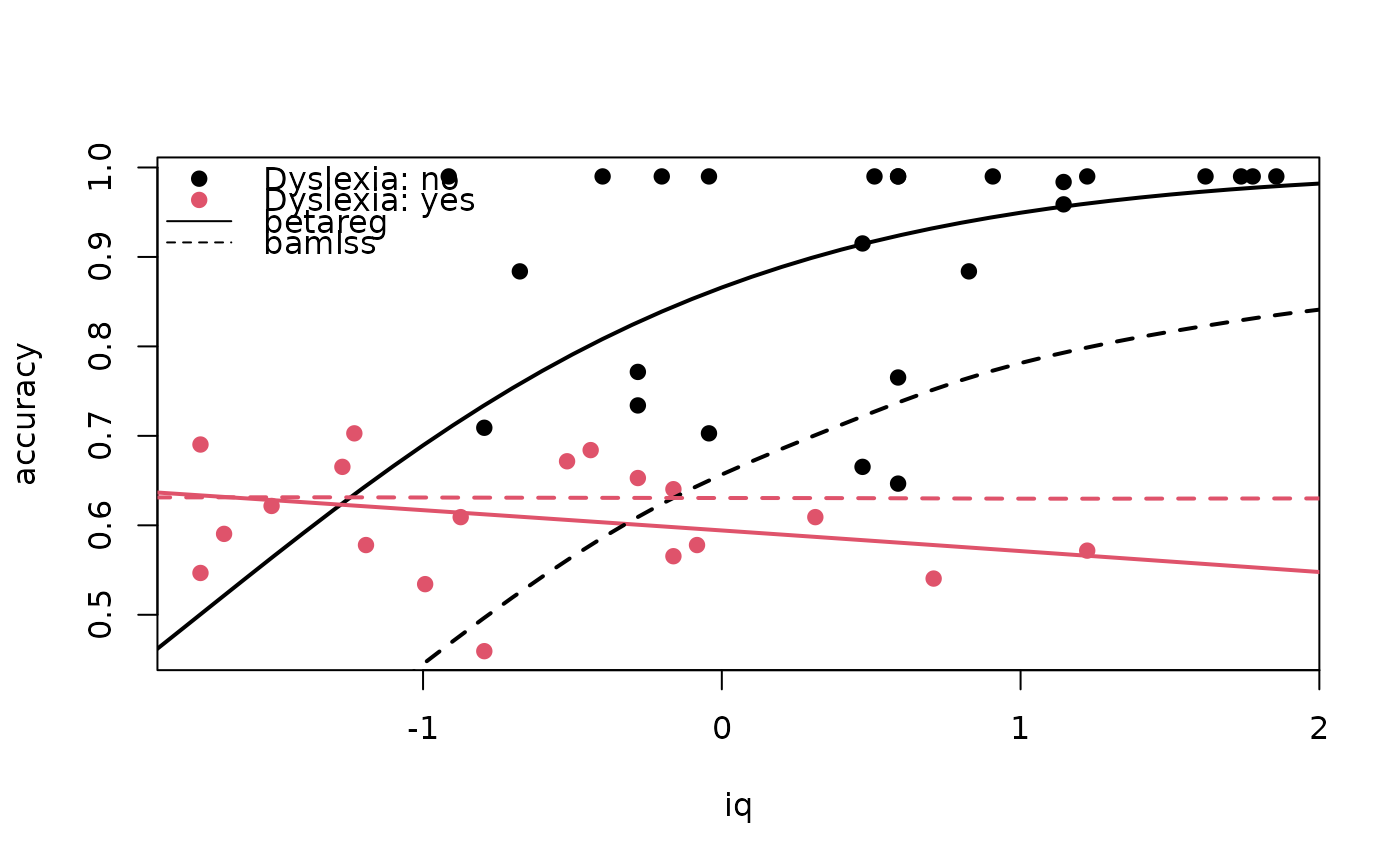
## Bayesian model shrinks the effects compared to ML
plot(accuracy ~ iq, data = ReadingSkills, pch = 19, col = dyslexia)
nd <- data.frame(
iq = rep(-19:20/10, 2),
dyslexia = factor(rep(c("no", "yes"), each = 40), levels = c("no", "yes"))
)
nd$betareg <- predict(rs1, newdata = nd, type = "response")
nd$bamlss <- predict(rs2, newdata = nd, type = "parameter", model = "mu")
lines(betareg ~ iq, data = nd, subset = dyslexia == "no", col = 1, lwd = 2, lty = 1)
lines(betareg ~ iq, data = nd, subset = dyslexia == "yes", col = 2, lwd = 2, lty = 1)
lines(bamlss ~ iq, data = nd, subset = dyslexia == "no", col = 1, lwd = 2, lty = 2)
lines(bamlss ~ iq, data = nd, subset = dyslexia == "yes", col = 2, lwd = 2, lty = 2)
legend("topleft", c("Dyslexia: no", "Dyslexia: yes", "betareg", "bamlss"),
lty = c(0, 0, 1, 2), pch = c(19, 19, NA, NA), col = c(1, 2, 1, 1), bty = "n")
 ## IGNORE_RDIFF_END
## xbetax_family(): requires more time due to Gaussian quadrature
## for gamlss2: install.packages("gamlss2", repos = "https://gamlss-dev.R-universe.dev")
## IGNORE_RDIFF_END
## xbetax_family(): requires more time due to Gaussian quadrature
## for gamlss2: install.packages("gamlss2", repos = "https://gamlss-dev.R-universe.dev")