Diagnostic Plots for betareg Objects
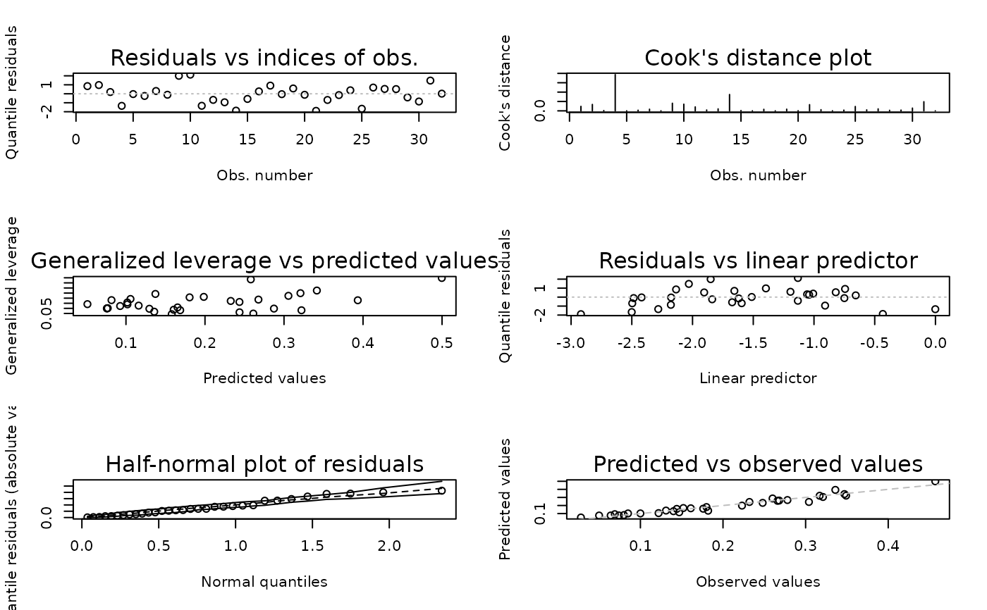
plot.betareg.RdVarious types of standard diagnostic plots can be produced, involving various types of residuals, influence measures etc.
Usage
# S3 method for class 'betareg'
plot(x, which = 1:4,
  caption = c("Residuals vs indices of obs.", "Cook's distance plot",
    "Generalized leverage vs predicted values", "Residuals vs linear predictor",
    "Half-normal plot of residuals", "Predicted vs observed values"),
    sub.caption = paste(deparse(x$call), collapse = "\n"), main = "",
    ask = prod(par("mfcol")) < length(which) && dev.interactive(),
    ..., type = "quantile", nsim = 100, level = 0.9)
Arguments
- x
fitted model object of class
"betareg".- which
numeric. If a subset of the plots is required, specify a subset of the numbers
1:6.- caption
character. Captions to appear above the plots.
- sub.caption
character. Common title-above figures if there are multiple.
- main
character. Title to each plot in addition to the above
caption.- ask
logical. If
TRUE, the user is asked before each plot.- ...
other parameters to be passed through to plotting functions.
- type
character indicating type of residual to be used, see
residuals.betareg.- nsim
numeric. Number of simulations in half-normal plots.
- level
numeric. Confidence level in half-normal plots.
Details
The plot method for betareg objects produces various types
of diagnostic plots. Most of these are standard for regression models and involve
various types of residuals, influence measures etc. See Ferrari and Cribari-Neto (2004)
for a discussion of some of these displays.
The which argument can be used to select a subset of currently six supported
types of displays. The corresponding element of caption contains a brief
description. In some more detail, the displays are: Residuals (as selected by
type) vs indices of observations (which = 1). Cook's distances
vs indices of observations (which = 2). Generalized leverage vs
predicted values (which = 3). Residuals vs linear predictor (which = 4).
Half-normal plot of residuals (which = 5), which is obtained using a simulation
approach. Predicted vs observed values (which = 6).
References
Cribari-Neto F, Zeileis A (2010). Beta Regression in R. Journal of Statistical Software, 34(2), 1–24. doi:10.18637/jss.v034.i02
Ferrari SLP, Cribari-Neto F (2004). Beta Regression for Modeling Rates and Proportions. Journal of Applied Statistics, 31(7), 799–815.