Tidy summarizes information about the components of a model. A model component might be a single term in a regression, a single hypothesis, a cluster, or a class. Exactly what tidy considers to be a model component varies across models but is usually self-evident. If a model has several distinct types of components, you will need to specify which components to return.
# S3 method for class 'lsmobj'
tidy(x, conf.int = FALSE, conf.level = 0.95, ...)
Arguments
- x
An
lsmobjobject.- conf.int
Logical indicating whether or not to include a confidence interval in the tidied output. Defaults to
FALSE.- conf.level
The confidence level to use for the confidence interval if
conf.int = TRUE. Must be strictly greater than 0 and less than 1. Defaults to 0.95, which corresponds to a 95 percent confidence interval.- ...
Additional arguments passed to
emmeans::summary.emmGrid()orlsmeans::summary.ref.grid(). Cautionary note: misspecified arguments may be silently ignored!
Details
Returns a data frame with one observation for each estimated marginal mean, and one column for each combination of factors. When the input is a contrast, each row will contain one estimated contrast.
There are a large number of arguments that can be
passed on to emmeans::summary.emmGrid() or lsmeans::summary.ref.grid().
See also
tidy(), emmeans::ref_grid(), emmeans::emmeans(),
emmeans::contrast()
Other emmeans tidiers:
tidy.emmGrid(),
tidy.ref.grid(),
tidy.summary_emm()
Value
A tibble::tibble() with columns:
- conf.high
Upper bound on the confidence interval for the estimate.
- conf.low
Lower bound on the confidence interval for the estimate.
- contrast
Levels being compared.
- df
Degrees of freedom used by this term in the model.
- null.value
Value to which the estimate is compared.
- p.value
The two-sided p-value associated with the observed statistic.
- std.error
The standard error of the regression term.
- estimate
Expected marginal mean
- statistic
T-ratio statistic
Examples
# load libraries for models and data
library(emmeans)
# linear model for sales of oranges per day
oranges_lm1 <- lm(sales1 ~ price1 + price2 + day + store, data = oranges)
# reference grid; see vignette("basics", package = "emmeans")
oranges_rg1 <- ref_grid(oranges_lm1)
td <- tidy(oranges_rg1)
td
#> # A tibble: 36 × 9
#> price1 price2 day store estimate std.error df statistic p.value
#> <dbl> <dbl> <chr> <chr> <dbl> <dbl> <dbl> <dbl> <dbl>
#> 1 51.2 48.6 1 1 2.92 2.72 23 1.07 0.294
#> 2 51.2 48.6 2 1 3.85 2.70 23 1.42 0.168
#> 3 51.2 48.6 3 1 11.0 2.53 23 4.35 0.000237
#> 4 51.2 48.6 4 1 6.10 2.65 23 2.30 0.0309
#> 5 51.2 48.6 5 1 12.8 3.43 23 3.73 0.00109
#> 6 51.2 48.6 6 1 8.75 3.59 23 2.44 0.0229
#> 7 51.2 48.6 1 2 4.96 3.12 23 1.59 0.125
#> 8 51.2 48.6 2 2 5.89 2.76 23 2.13 0.0438
#> 9 51.2 48.6 3 2 13.1 2.74 23 4.77 0.0000823
#> 10 51.2 48.6 4 2 8.14 2.74 23 2.97 0.00692
#> # ℹ 26 more rows
# marginal averages
marginal <- emmeans(oranges_rg1, "day")
tidy(marginal)
#> # A tibble: 6 × 6
#> day estimate std.error df statistic p.value
#> <chr> <dbl> <dbl> <dbl> <dbl> <dbl>
#> 1 1 5.56 2.09 23 2.66 0.0140
#> 2 2 6.49 1.84 23 3.53 0.00180
#> 3 3 13.7 1.82 23 7.50 0.000000128
#> 4 4 8.74 1.83 23 4.77 0.0000822
#> 5 5 15.4 3.20 23 4.83 0.0000712
#> 6 6 11.4 3.08 23 3.70 0.00118
# contrasts
tidy(contrast(marginal))
#> # A tibble: 6 × 8
#> term contrast null.value estimate std.error df statistic adj.p.value
#> <chr> <chr> <dbl> <dbl> <dbl> <dbl> <dbl> <dbl>
#> 1 day day1 effect 0 -4.65 1.35 23 -3.45 0.0131
#> 2 day day2 effect 0 -3.72 1.82 23 -2.05 0.105
#> 3 day day3 effect 0 3.45 1.82 23 1.89 0.106
#> 4 day day4 effect 0 -1.47 1.84 23 -0.800 0.518
#> 5 day day5 effect 0 5.22 1.88 23 2.77 0.0324
#> 6 day day6 effect 0 1.18 2.24 23 0.525 0.605
tidy(contrast(marginal, method = "pairwise"))
#> # A tibble: 15 × 8
#> term contrast null.value estimate std.error df statistic adj.p.value
#> <chr> <chr> <dbl> <dbl> <dbl> <dbl> <dbl> <dbl>
#> 1 day day1 - day2 0 -0.930 2.47 23 -0.377 0.999
#> 2 day day1 - day3 0 -8.10 2.47 23 -3.29 0.0337
#> 3 day day1 - day4 0 -3.18 2.51 23 -1.27 0.799
#> 4 day day1 - day5 0 -9.88 2.56 23 -3.86 0.00913
#> 5 day day1 - day6 0 -5.83 2.52 23 -2.31 0.229
#> 6 day day2 - day3 0 -7.17 2.48 23 -2.89 0.0777
#> 7 day day2 - day4 0 -2.25 2.44 23 -0.920 0.937
#> 8 day day2 - day5 0 -8.95 3.08 23 -2.90 0.0761
#> 9 day day2 - day6 0 -4.90 3.54 23 -1.38 0.737
#> 10 day day3 - day4 0 4.92 2.49 23 1.98 0.385
#> 11 day day3 - day5 0 -1.78 3.08 23 -0.578 0.992
#> 12 day day3 - day6 0 2.27 3.52 23 0.644 0.986
#> 13 day day4 - day5 0 -6.70 3.11 23 -2.16 0.295
#> 14 day day4 - day6 0 -2.65 3.57 23 -0.744 0.974
#> 15 day day5 - day6 0 4.05 2.56 23 1.58 0.617
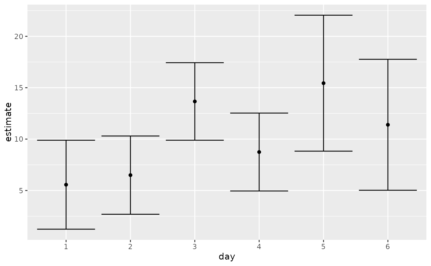
# plot confidence intervals
library(ggplot2)
ggplot(tidy(marginal, conf.int = TRUE), aes(day, estimate)) +
geom_point() +
geom_errorbar(aes(ymin = conf.low, ymax = conf.high))
 # by multiple prices
by_price <- emmeans(oranges_lm1, "day",
by = "price2",
at = list(
price1 = 50, price2 = c(40, 60, 80),
day = c("2", "3", "4")
)
)
by_price
#> price2 = 40:
#> day emmean SE df lower.CL upper.CL
#> 2 6.24 1.93 23 2.24 10.2
#> 3 13.41 2.13 23 9.00 17.8
#> 4 8.48 1.90 23 4.55 12.4
#>
#> price2 = 60:
#> day emmean SE df lower.CL upper.CL
#> 2 9.21 2.23 23 4.59 13.8
#> 3 16.38 2.01 23 12.23 20.5
#> 4 11.46 2.29 23 6.73 16.2
#>
#> price2 = 80:
#> day emmean SE df lower.CL upper.CL
#> 2 12.19 3.77 23 4.40 20.0
#> 3 19.36 3.39 23 12.35 26.4
#> 4 14.44 3.85 23 6.48 22.4
#>
#> Results are averaged over the levels of: store
#> Confidence level used: 0.95
tidy(by_price)
#> # A tibble: 9 × 7
#> day price2 estimate std.error df statistic p.value
#> <chr> <dbl> <dbl> <dbl> <dbl> <dbl> <dbl>
#> 1 2 40 6.24 1.93 23 3.22 0.00375
#> 2 3 40 13.4 2.13 23 6.30 0.00000199
#> 3 4 40 8.48 1.90 23 4.46 0.000178
#> 4 2 60 9.21 2.23 23 4.13 0.000411
#> 5 3 60 16.4 2.01 23 8.17 0.0000000300
#> 6 4 60 11.5 2.29 23 5.01 0.0000455
#> 7 2 80 12.2 3.77 23 3.24 0.00365
#> 8 3 80 19.4 3.39 23 5.71 0.00000807
#> 9 4 80 14.4 3.85 23 3.75 0.00104
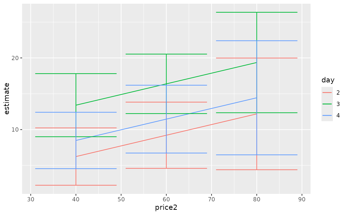
ggplot(tidy(by_price, conf.int = TRUE), aes(price2, estimate, color = day)) +
geom_line() +
geom_errorbar(aes(ymin = conf.low, ymax = conf.high))
# by multiple prices
by_price <- emmeans(oranges_lm1, "day",
by = "price2",
at = list(
price1 = 50, price2 = c(40, 60, 80),
day = c("2", "3", "4")
)
)
by_price
#> price2 = 40:
#> day emmean SE df lower.CL upper.CL
#> 2 6.24 1.93 23 2.24 10.2
#> 3 13.41 2.13 23 9.00 17.8
#> 4 8.48 1.90 23 4.55 12.4
#>
#> price2 = 60:
#> day emmean SE df lower.CL upper.CL
#> 2 9.21 2.23 23 4.59 13.8
#> 3 16.38 2.01 23 12.23 20.5
#> 4 11.46 2.29 23 6.73 16.2
#>
#> price2 = 80:
#> day emmean SE df lower.CL upper.CL
#> 2 12.19 3.77 23 4.40 20.0
#> 3 19.36 3.39 23 12.35 26.4
#> 4 14.44 3.85 23 6.48 22.4
#>
#> Results are averaged over the levels of: store
#> Confidence level used: 0.95
tidy(by_price)
#> # A tibble: 9 × 7
#> day price2 estimate std.error df statistic p.value
#> <chr> <dbl> <dbl> <dbl> <dbl> <dbl> <dbl>
#> 1 2 40 6.24 1.93 23 3.22 0.00375
#> 2 3 40 13.4 2.13 23 6.30 0.00000199
#> 3 4 40 8.48 1.90 23 4.46 0.000178
#> 4 2 60 9.21 2.23 23 4.13 0.000411
#> 5 3 60 16.4 2.01 23 8.17 0.0000000300
#> 6 4 60 11.5 2.29 23 5.01 0.0000455
#> 7 2 80 12.2 3.77 23 3.24 0.00365
#> 8 3 80 19.4 3.39 23 5.71 0.00000807
#> 9 4 80 14.4 3.85 23 3.75 0.00104
ggplot(tidy(by_price, conf.int = TRUE), aes(price2, estimate, color = day)) +
geom_line() +
geom_errorbar(aes(ymin = conf.low, ymax = conf.high))
 # joint_tests
tidy(joint_tests(oranges_lm1))
#> # A tibble: 4 × 5
#> term num.df den.df statistic p.value
#> <chr> <dbl> <dbl> <dbl> <dbl>
#> 1 price1 1 23 30.3 0.0000134
#> 2 price2 1 23 2.23 0.149
#> 3 day 5 23 4.95 0.00321
#> 4 store 5 23 2.52 0.0583
# joint_tests
tidy(joint_tests(oranges_lm1))
#> # A tibble: 4 × 5
#> term num.df den.df statistic p.value
#> <chr> <dbl> <dbl> <dbl> <dbl>
#> 1 price1 1 23 30.3 0.0000134
#> 2 price2 1 23 2.23 0.149
#> 3 day 5 23 4.95 0.00321
#> 4 store 5 23 2.52 0.0583