Fast Growth Rates for Time Series and Panel Data
fgrowth.Rdfgrowth is a S3 generic to compute (sequences of) suitably lagged / leaded, iterated and compounded growth rates, obtained with via the exact method of computation or through log differencing. By default growth rates are provided in percentage terms, but any scale factor can be applied. The growth operator G is a parsimonious wrapper around fgrowth, and also provides more flexibility when applied to data frames.
fgrowth(x, n = 1, diff = 1, ...)
      G(x, n = 1, diff = 1, ...)

# Default S3 method
fgrowth(x, n = 1, diff = 1, g = NULL, t = NULL, fill = NA,
        logdiff = FALSE, scale = 100, power = 1, stubs = TRUE, ...)
# Default S3 method
G(x, n = 1, diff = 1, g = NULL, t = NULL, fill = NA, logdiff = FALSE,
  scale = 100, power = 1, stubs = .op[["stub"]], ...)

# S3 method for class 'matrix'
fgrowth(x, n = 1, diff = 1, g = NULL, t = NULL, fill = NA,
        logdiff = FALSE, scale = 100, power = 1,
        stubs = length(n) + length(diff) > 2L, ...)
# S3 method for class 'matrix'
G(x, n = 1, diff = 1, g = NULL, t = NULL, fill = NA, logdiff = FALSE,
  scale = 100, power = 1, stubs = .op[["stub"]], ...)

# S3 method for class 'data.frame'
fgrowth(x, n = 1, diff = 1, g = NULL, t = NULL, fill = NA,
        logdiff = FALSE, scale = 100, power = 1,
        stubs = length(n) + length(diff) > 2L, ...)
# S3 method for class 'data.frame'
G(x, n = 1, diff = 1, by = NULL, t = NULL, cols = is.numeric,
  fill = NA, logdiff = FALSE, scale = 100, power = 1, stubs = .op[["stub"]],
  keep.ids = TRUE, ...)

# Methods for indexed data / compatibility with plm:

# S3 method for class 'pseries'
fgrowth(x, n = 1, diff = 1, fill = NA, logdiff = FALSE, scale = 100,
        power = 1, stubs = length(n) + length(diff) > 2L, shift = "time", ...)
# S3 method for class 'pseries'
G(x, n = 1, diff = 1, fill = NA, logdiff = FALSE, scale = 100,
  power = 1, stubs = .op[["stub"]], shift = "time", ...)

# S3 method for class 'pdata.frame'
fgrowth(x, n = 1, diff = 1, fill = NA, logdiff = FALSE, scale = 100,
        power = 1, stubs = length(n) + length(diff) > 2L, shift = "time", ...)
# S3 method for class 'pdata.frame'
G(x, n = 1, diff = 1, cols = is.numeric, fill = NA, logdiff = FALSE,
  scale = 100, power = 1, stubs = .op[["stub"]], shift = "time", keep.ids = TRUE, ...)

# Methods for grouped data frame / compatibility with dplyr:

# S3 method for class 'grouped_df'
fgrowth(x, n = 1, diff = 1, t = NULL, fill = NA, logdiff = FALSE,
        scale = 100, power = 1, stubs = length(n) + length(diff) > 2L,
        keep.ids = TRUE, ...)
# S3 method for class 'grouped_df'
G(x, n = 1, diff = 1, t = NULL, fill = NA, logdiff = FALSE,
  scale = 100, power = 1, stubs = .op[["stub"]], keep.ids = TRUE, ...)
Arguments
- x
a numeric vector / time series, (time series) matrix, data frame, 'indexed_series' ('pseries'), 'indexed_frame' ('pdata.frame') or grouped data frame ('grouped_df').
- n
integer. A vector indicating the number of lags or leads.
- diff
integer. A vector of integers > 1 indicating the order of taking growth rates, e.g.
diff = 2means computing the growth rate of the growth rate.- g
a factor,
GRPobject, or atomic vector / list of vectors (internally grouped withgroup) used to groupx. Note that withoutt, all values in a group need to be consecutive and in the right order. See Details offlag.- by
data.frame method: Same as
g, but also allows one- or two-sided formulas i.e.~ group1orvar1 + var2 ~ group1 + group2. See Examples.- t
a time vector or list of vectors. See
flag.- cols
data.frame method: Select columns to compute growth rates using a function, column names, indices or a logical vector. Default: All numeric variables. Note:
colsis ignored if a two-sided formula is passed toby.- fill
value to insert when vectors are shifted. Default is
NA.- logdiff
logical. Compute log-difference growth rates instead of exact growth rates. See Details.
- scale
logical. Scale factor post-applied to growth rates, default is 100 which gives growth rates in percentage terms. See Details.
- power
numeric. Apply a power to annualize or compound growth rates e.g.
fgrowth(AirPassengers, 12, power = 1/12)is equivalent to((AirPassengers/flag(AirPassengers, 12))^(1/12)-1)*100.- stubs
logical.
TRUE(default) will rename all computed columns by adding a prefix "LnGdiff." / "FnGdiff.", or "LnDlogdiff." / "FnDlogdiff." iflogdiff = TRUE.- shift
pseries / pdata.frame methods: character.
"time"or"row". Seeflagfor details.- keep.ids
data.frame / pdata.frame / grouped_df methods: Logical. Drop all identifiers from the output (which includes all variables passed to
byortusing formulas). Note: For 'grouped_df' / 'pdata.frame' identifiers are dropped, but the"groups"/"index"attributes are kept.- ...
arguments to be passed to or from other methods.
Details
fgrowth/G by default computes exact growth rates using repeat(diff) ((x[i]/x[i-n])^power - 1)*scale, so for diff > 1 it computes growth rate of growth rates. If logdiff = TRUE, approximate growth rates are computed using log(x[i]/x[i-n])*scale for diff = 1 and repeat(diff-1) x[i] - x[i-n] thereafter (usually diff = 1 for log-differencing). For further details see the help pages of fdiff and flag.
Value
x where the growth rate was taken diff times using lags n of itself, scaled by scale. Computations can be grouped by g/by and/or ordered by t. See Details and Examples.
Examples
## Simple Time Series: AirPassengers
G(AirPassengers) # Growth rate, same as fgrowth(AirPassengers)
#> Jan Feb Mar Apr May Jun
#> 1949 NA 5.3571429 11.8644068 -2.2727273 -6.2015504 11.5702479
#> 1950 -2.5423729 9.5652174 11.9047619 -4.2553191 -7.4074074 19.2000000
#> 1951 3.5714286 3.4482759 18.6666667 -8.4269663 5.5214724 3.4883721
#> 1952 3.0120482 5.2631579 7.2222222 -6.2176166 1.1049724 19.1256831
#> 1953 1.0309278 0.0000000 20.4081633 -0.4237288 -2.5531915 6.1135371
#> 1954 1.4925373 -7.8431373 25.0000000 -3.4042553 3.0837004 12.8205128
#> 1955 5.6768559 -3.7190083 14.5922747 0.7490637 0.3717472 16.6666667
#> 1956 2.1582734 -2.4647887 14.4404332 -1.2618297 1.5974441 17.6100629
#> 1957 2.9411765 -4.4444444 18.2724252 -2.2471910 2.0114943 18.8732394
#> 1958 1.1904762 -6.4705882 13.8364780 -3.8674033 4.3103448 19.8347107
#> 1959 6.8249258 -5.0000000 18.7134503 -2.4630542 6.0606061 12.3809524
#> 1960 2.9629630 -6.2350120 7.1611253 10.0238663 2.3861171 13.3474576
#> Jul Aug Sep Oct Nov Dec
#> 1949 9.6296296 0.0000000 -8.1081081 -12.5000000 -12.6050420 13.4615385
#> 1950 14.0939597 0.0000000 -7.0588235 -15.8227848 -14.2857143 22.8070175
#> 1951 11.7977528 0.0000000 -7.5376884 -11.9565217 -9.8765432 13.6986301
#> 1952 5.5045872 5.2173913 -13.6363636 -8.6124402 -9.9476440 12.7906977
#> 1953 8.6419753 3.0303030 -12.8676471 -10.9704641 -14.6919431 11.6666667
#> 1954 14.3939394 -2.9801325 -11.6040956 -11.5830116 -11.3537118 12.8078818
#> 1955 15.5555556 -4.6703297 -10.0864553 -12.1794872 -13.5036496 17.2995781
#> 1956 10.4278075 -1.9370460 -12.3456790 -13.8028169 -11.4379085 12.9151292
#> 1957 10.1895735 0.4301075 -13.4903640 -14.1089109 -12.1037464 10.1639344
#> 1958 12.8735632 2.8513238 -20.0000000 -11.1386139 -13.6490251 8.7096774
#> 1959 16.1016949 2.0072993 -17.1735242 -12.0950324 -11.0565111 11.8784530
#> 1960 16.2616822 -2.5723473 -16.1716172 -9.2519685 -15.4013015 10.7692308
G(AirPassengers, logdiff = TRUE) # Log-difference
#> Jan Feb Mar Apr May Jun
#> 1949 NA 5.2185753 11.2117298 -2.2989518 -6.4021859 10.9484233
#> 1950 -2.5752496 9.1349779 11.2477983 -4.3485112 -7.6961041 17.5632569
#> 1951 3.5091320 3.3901552 17.1148256 -8.8033349 5.3744276 3.4289073
#> 1952 2.9675768 5.1293294 6.9733338 -6.4193158 1.0989122 17.5008910
#> 1953 1.0256500 0.0000000 18.5717146 -0.4246291 -2.5863511 5.9339440
#> 1954 1.4815086 -8.1678031 22.3143551 -3.4635497 3.0371098 12.0627988
#> 1955 5.5215723 -3.7899273 13.6210205 0.7462721 0.3710579 15.4150680
#> 1956 2.1353124 -2.4956732 13.4884268 -1.2698583 1.5848192 16.2204415
#> 1957 2.8987537 -4.5462374 16.7820466 -2.2728251 1.9915310 17.2887525
#> 1958 1.1834458 -6.6894235 12.9592829 -3.9441732 4.2200354 18.0943197
#> 1959 6.6021101 -5.1293294 17.1542423 -2.4938948 5.8840500 11.6724274
#> 1960 2.9199155 -6.4378662 6.9163360 9.5527123 2.3580943 12.5287761
#> Jul Aug Sep Oct Nov Dec
#> 1949 9.1937495 0.0000000 -8.4557388 -13.3531393 -13.4732594 12.6293725
#> 1950 13.1852131 0.0000000 -7.3203404 -17.2245905 -15.4150680 20.5443974
#> 1951 11.1521274 0.0000000 -7.8369067 -12.7339422 -10.3989714 12.8381167
#> 1952 5.3584246 5.0858417 -14.6603474 -9.0060824 -10.4778951 12.0363682
#> 1953 8.2887660 2.9852963 -13.7741925 -11.6202008 -15.8901283 11.0348057
#> 1954 13.4477914 -3.0254408 -12.3344547 -12.3106058 -12.0516025 12.0516025
#> 1955 14.4581229 -4.7829088 -10.6321592 -12.9875081 -14.5067965 15.9560973
#> 1956 9.9191796 -1.9560526 -13.1769278 -14.8532688 -12.1466281 12.1466281
#> 1957 9.7032092 0.4291852 -14.4914380 -15.2090098 -12.9013003 9.6799383
#> 1958 12.1098097 2.8114301 -22.3143551 -11.8092489 -14.6750091 8.3510633
#> 1959 14.9296301 1.9874186 -18.8422419 -12.8913869 -11.7168974 11.2242855
#> 1960 15.0673346 -2.6060107 -17.6398538 -9.7083405 -16.7251304 10.2278849
G(AirPassengers, 1, 2) # Growth rate of growth rate
#> Jan Feb Mar Apr May
#> 1949 NA NA 121.4689266 -119.1558442 172.8682171
#> 1950 -118.8861985 -476.2318841 24.4588745 -135.7446809 74.0740741
#> 1951 -84.3406593 -3.4482759 441.3333333 -145.1444623 -165.5214724
#> 1952 -78.0120482 74.7368421 37.2222222 -186.0900757 -117.7716390
#> 1953 -91.9400187 -100.0000000 Inf -102.0762712 502.5531915
#> 1954 -87.2068230 -625.4901961 -418.7500000 -113.6170213 -190.5837004
#> 1955 -55.6768559 -165.5117610 -492.3700525 -94.8667107 -50.3717472
#> 1956 -87.5241270 -214.2018779 -685.8690046 -108.7381703 -226.5974441
#> 1957 -77.2268908 -251.1111111 -511.1295681 -112.2982635 -189.5114943
#> 1958 -88.2872504 -643.5294118 -313.8364780 -127.9507785 -211.4532020
#> 1959 -21.6397406 -173.2608696 -474.2690058 -113.1619458 -346.0606061
#> 1960 -75.0559862 -310.4316547 -214.8534330 39.9761337 -76.1956409
#> Jun Jul Aug Sep Oct
#> 1949 -286.5702479 -16.7724868 -100.0000000 -Inf 54.1666667
#> 1950 -359.2000000 -26.5939597 -100.0000000 -Inf 124.1561181
#> 1951 -36.8217054 238.2022472 -100.0000000 -Inf 58.6231884
#> 1952 1630.8743169 -71.2188729 -5.2173913 -361.3636364 -36.8421053
#> 1953 -339.4468705 41.3580247 -64.9350649 -524.6323529 -14.7438216
#> 1954 315.7509158 12.2727273 -120.7040781 289.3818733 -0.1816943
#> 1955 4383.3333333 -6.6666667 -130.0235479 115.9688083 20.7509158
#> 1956 1002.3899371 -40.7849503 -118.5757745 537.3456790 11.8028169
#> 1957 838.2696177 -46.0104690 -95.7789447 -3236.5096360 4.5851014
#> 1958 360.1652893 -35.0957854 -77.8513238 -801.4285714 -44.3069307
#> 1959 104.2857143 30.0521512 -87.5336151 -955.5537486 -29.5716343
#> 1960 459.3798151 21.8335559 -115.8184573 528.6716172 -42.7888478
#> Nov Dec
#> 1949 0.8403361 -206.7948718
#> 1950 -9.7142857 -259.6491228
#> 1951 -17.3961841 -238.6986301
#> 1952 15.5031995 -228.5801714
#> 1953 33.9227124 -179.4086022
#> 1954 -1.9796215 -212.8078818
#> 1955 10.8720707 -228.1103889
#> 1956 -17.1335201 -212.9151292
#> 1957 -14.2120431 -183.9734582
#> 1958 22.5379140 -163.8117182
#> 1959 -8.5863461 -207.4340086
#> 1960 66.4651313 -169.9241603
G(AirPassengers, 12) # Seasonal growth rate (data is monthly)
#> Jan Feb Mar Apr May Jun
#> 1949 NA NA NA NA NA NA
#> 1950 2.6785714 6.7796610 6.8181818 4.6511628 3.3057851 10.3703704
#> 1951 26.0869565 19.0476190 26.2411348 20.7407407 37.6000000 19.4630872
#> 1952 17.9310345 20.0000000 8.4269663 11.0429448 6.3953488 22.4719101
#> 1953 14.6198830 8.8888889 22.2797927 29.8342541 25.1366120 11.4678899
#> 1954 4.0816327 -4.0816327 -0.4237288 -3.4042553 2.1834061 8.6419753
#> 1955 18.6274510 23.9361702 13.6170213 18.5022026 15.3846154 19.3181818
#> 1956 17.3553719 18.8841202 18.7265918 16.3568773 17.7777778 18.7301587
#> 1957 10.9154930 8.6642599 12.3028391 11.1821086 11.6352201 12.8342246
#> 1958 7.9365079 5.6478405 1.6853933 0.0000000 2.2535211 3.0805687
#> 1959 5.8823529 7.5471698 12.1546961 13.7931034 15.7024793 8.5057471
#> 1960 15.8333333 14.3274854 3.2019704 16.4141414 12.3809524 13.3474576
#> Jul Aug Sep Oct Nov Dec
#> 1949 NA NA NA NA NA NA
#> 1950 14.8648649 14.8648649 16.1764706 11.7647059 9.6153846 18.6440678
#> 1951 17.0588235 17.0588235 16.4556962 21.8045113 28.0701754 18.5714286
#> 1952 15.5778894 21.6080402 13.5869565 17.9012346 17.8082192 16.8674699
#> 1953 14.7826087 12.3966942 13.3971292 10.4712042 4.6511628 3.6082474
#> 1954 14.3939394 7.7205882 9.2827004 8.5308057 12.7777778 13.9303483
#> 1955 20.5298013 18.4300341 20.4633205 19.6506550 16.7487685 21.3973799
#> 1956 13.4615385 16.7146974 13.7820513 11.6788321 14.3459916 10.0719424
#> 1957 12.5907990 15.3086420 13.8028169 13.3986928 12.5461255 9.8039216
#> 1958 5.5913978 8.1370450 0.0000000 3.4582133 1.6393443 0.2976190
#> 1959 11.6089613 10.6930693 14.6039604 13.3704735 16.7741935 20.1780415
#> 1960 13.5036496 8.4078712 9.7192225 13.2678133 7.7348066 6.6666667
head(G(AirPassengers, -2:2, 1:3)) # Sequence of leaded/lagged and iterated growth rates
#> F2G1 F2G2 F2G3 FG1 FG2 FG3 --
#> [1,] -15.151515 -266.66667 77.97753 -5.084746 -52.05811 -90.63805 112
#> [2,] -8.527132 91.86047 -285.94592 -10.606061 -556.06061 757.77959 118
#> [3,] 9.090909 -149.83165 -51.15620 2.325581 -64.82558 -60.41293 132
#> [4,] -4.444444 -49.40171 -63.68691 6.611570 -163.75443 -1006.58997 129
#> [5,] -18.243243 -306.75676 330.09195 -10.370370 18.06268 NaN 121
#> [6,] -8.783784 -136.04380 -104.90137 -8.783784 -Inf Inf 135
#> G1 G2 G3 L2G1 L2G2 L2G3
#> [1,] NA NA NA NA NA NA
#> [2,] 5.357143 NA NA NA NA NA
#> [3,] 11.864407 121.4689 NA 17.857143 NA NA
#> [4,] -2.272727 -119.1558 -198.0957 9.322034 NA NA
#> [5,] -6.201550 172.8682 -245.0774 -8.333333 -146.66667 NA
#> [6,] 11.570248 -286.5702 -265.7738 4.651163 -50.10571 NA
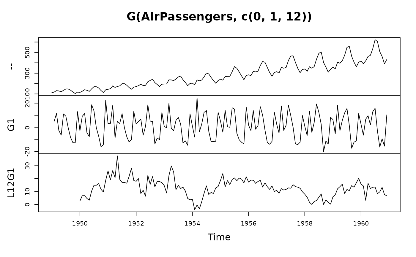
# let's do some visual analysis
plot(G(AirPassengers, c(0, 1, 12)))
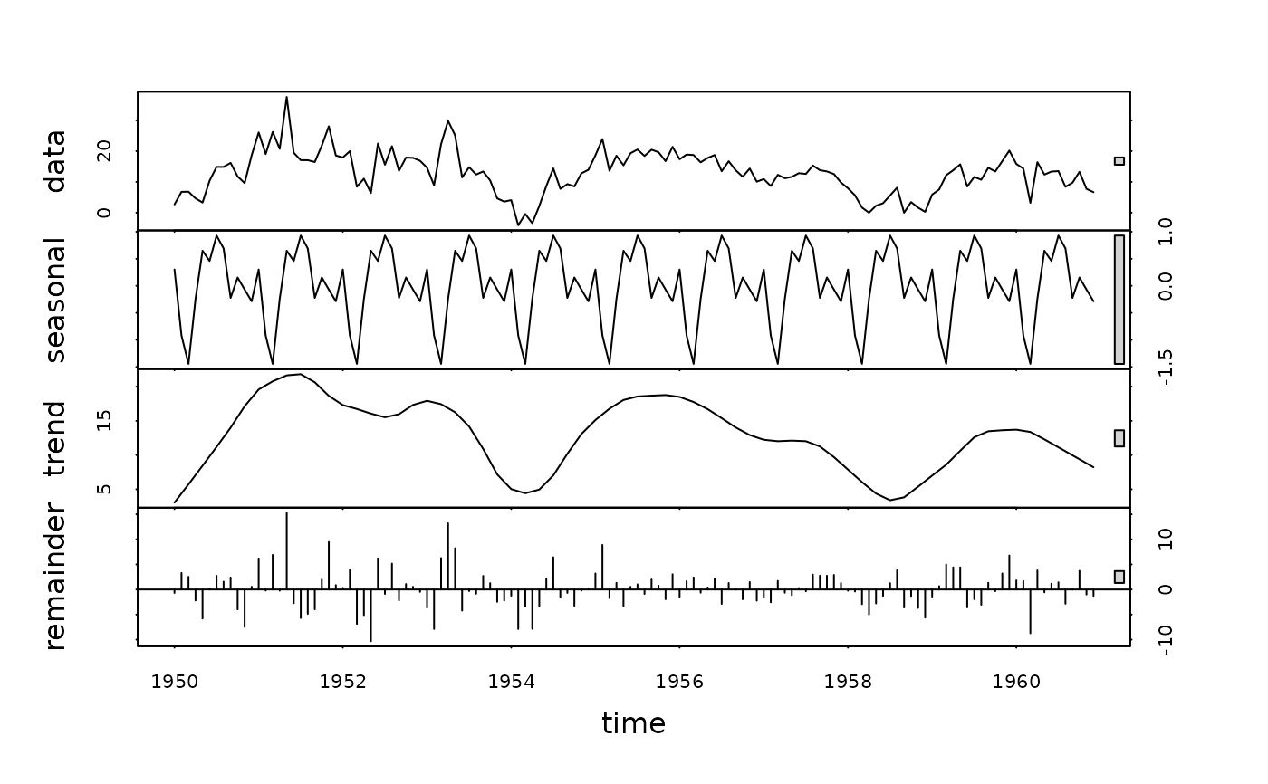
 plot(stl(window(G(AirPassengers, 12), # Taking seasonal growth rate removes most seasonal variation
1950), "periodic"))
plot(stl(window(G(AirPassengers, 12), # Taking seasonal growth rate removes most seasonal variation
1950), "periodic"))
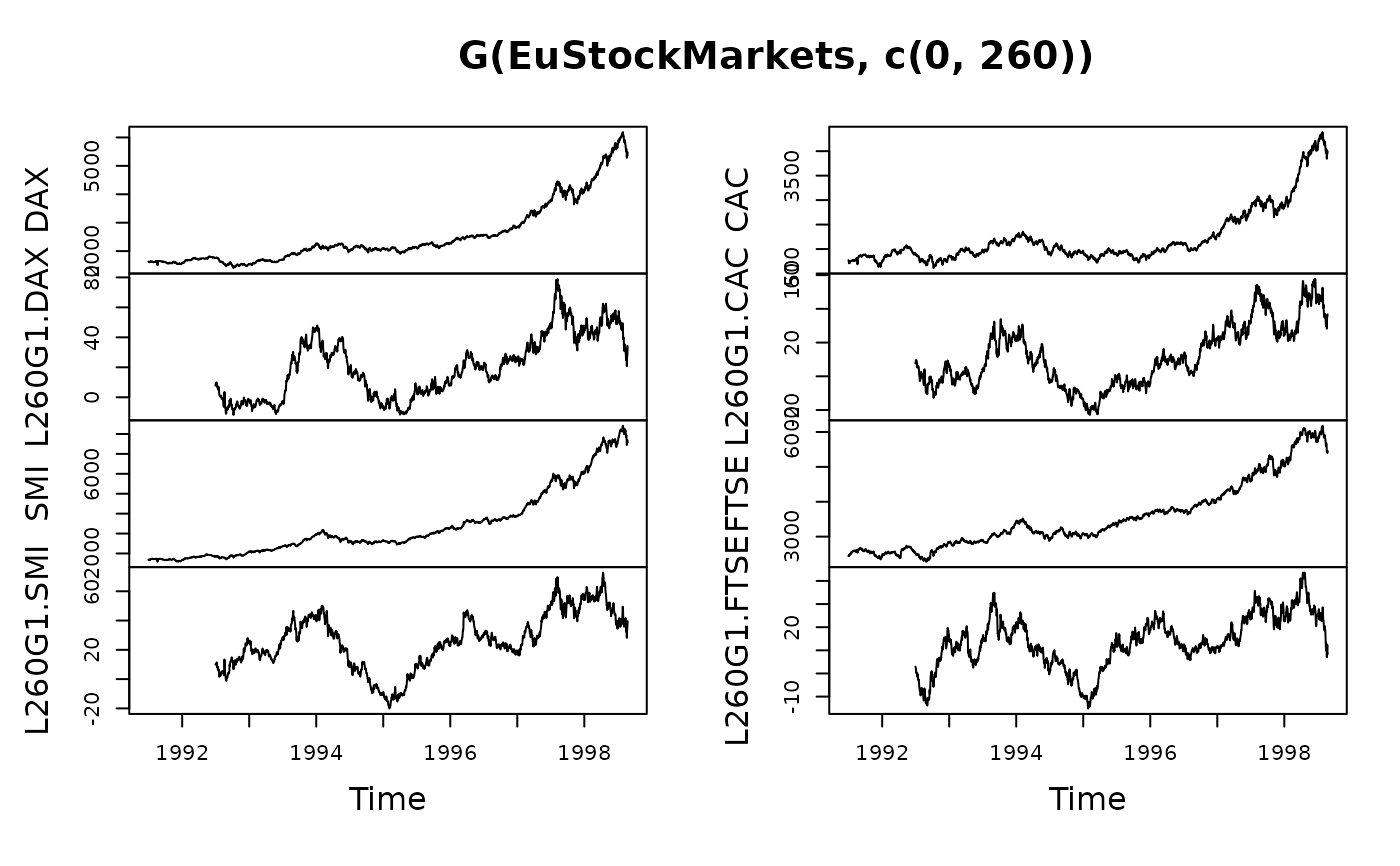
 ## Time Series Matrix of 4 EU Stock Market Indicators, recorded 260 days per year
plot(G(EuStockMarkets,c(0,260))) # Plot series and annual growth rates
## Time Series Matrix of 4 EU Stock Market Indicators, recorded 260 days per year
plot(G(EuStockMarkets,c(0,260))) # Plot series and annual growth rates
 summary(lm(L260G1.DAX ~., G(EuStockMarkets,260))) # Annual growth rate of DAX regressed on the
#>
#> Call:
#> lm(formula = L260G1.DAX ~ ., data = G(EuStockMarkets, 260))
#>
#> Residuals:
#> Min 1Q Median 3Q Max
#> -19.5094 -4.7763 0.4586 5.0337 18.2316
#>
#> Coefficients:
#> Estimate Std. Error t value Pr(>|t|)
#> (Intercept) 4.48795 0.38357 11.70 < 2e-16 ***
#> L260G1.SMI 0.37048 0.02635 14.06 < 2e-16 ***
#> L260G1.CAC 0.82319 0.02092 39.34 < 2e-16 ***
#> L260G1.FTSE -0.25008 0.03883 -6.44 1.58e-10 ***
#> ---
#> Signif. codes: 0 ‘***’ 0.001 ‘**’ 0.01 ‘*’ 0.05 ‘.’ 0.1 ‘ ’ 1
#>
#> Residual standard error: 7.817 on 1596 degrees of freedom
#> (260 observations deleted due to missingness)
#> Multiple R-squared: 0.8585, Adjusted R-squared: 0.8582
#> F-statistic: 3226 on 3 and 1596 DF, p-value: < 2.2e-16
#>
# growth rates of the other indicators
## World Development Panel Data
head(fgrowth(num_vars(wlddev), 1, 1, # Computes growth rates of numeric variables
wlddev$country, wlddev$year)) # fgrowth requires external inputs..
#> year decade PCGDP LIFEEX GINI ODA POP
#> 1 NA NA NA NA NA NA NA
#> 2 0.05102041 0 NA 1.590335 NA 98.74969 1.916611
#> 3 0.05099439 0 NA 1.544202 NA -51.37884 1.985199
#> 4 0.05096840 0 NA 1.493830 NA 110.66998 2.050636
#> 5 0.05094244 0 NA 1.448294 NA 24.48259 2.112246
#> 6 0.05091650 0 NA 1.407306 NA 15.51770 2.170793
head(G(wlddev, 1, 1, ~country, ~year)) # Growth of numeric variables, id's attached
#> country year G1.decade G1.PCGDP G1.LIFEEX G1.GINI G1.ODA G1.POP
#> 1 Afghanistan 1960 NA NA NA NA NA NA
#> 2 Afghanistan 1961 0 NA 1.590335 NA 98.74969 1.916611
#> 3 Afghanistan 1962 0 NA 1.544202 NA -51.37884 1.985199
#> 4 Afghanistan 1963 0 NA 1.493830 NA 110.66998 2.050636
#> 5 Afghanistan 1964 0 NA 1.448294 NA 24.48259 2.112246
#> 6 Afghanistan 1965 0 NA 1.407306 NA 15.51770 2.170793
head(G(wlddev, 1, 1, ~country)) # Without t: Works because data is ordered
#> country G1.year G1.decade G1.PCGDP G1.LIFEEX G1.GINI G1.ODA
#> 1 Afghanistan NA NA NA NA NA NA
#> 2 Afghanistan 0.05102041 0 NA 1.590335 NA 98.74969
#> 3 Afghanistan 0.05099439 0 NA 1.544202 NA -51.37884
#> 4 Afghanistan 0.05096840 0 NA 1.493830 NA 110.66998
#> 5 Afghanistan 0.05094244 0 NA 1.448294 NA 24.48259
#> 6 Afghanistan 0.05091650 0 NA 1.407306 NA 15.51770
#> G1.POP
#> 1 NA
#> 2 1.916611
#> 3 1.985199
#> 4 2.050636
#> 5 2.112246
#> 6 2.170793
head(G(wlddev, 1, 1, PCGDP + LIFEEX ~ country, ~year)) # Growth of GDP per Capita & Life Expectancy
#> country year G1.PCGDP G1.LIFEEX
#> 1 Afghanistan 1960 NA NA
#> 2 Afghanistan 1961 NA 1.590335
#> 3 Afghanistan 1962 NA 1.544202
#> 4 Afghanistan 1963 NA 1.493830
#> 5 Afghanistan 1964 NA 1.448294
#> 6 Afghanistan 1965 NA 1.407306
head(G(wlddev, 0:1, 1, ~ country, ~year, cols = 9:10)) # Same, also retaining original series
#> country year PCGDP G1.PCGDP LIFEEX G1.LIFEEX
#> 1 Afghanistan 1960 NA NA 32.446 NA
#> 2 Afghanistan 1961 NA NA 32.962 1.590335
#> 3 Afghanistan 1962 NA NA 33.471 1.544202
#> 4 Afghanistan 1963 NA NA 33.971 1.493830
#> 5 Afghanistan 1964 NA NA 34.463 1.448294
#> 6 Afghanistan 1965 NA NA 34.948 1.407306
head(G(wlddev, 0:1, 1, ~ country, ~year, 9:10, # Dropping id columns
keep.ids = FALSE))
#> PCGDP G1.PCGDP LIFEEX G1.LIFEEX
#> 1 NA NA 32.446 NA
#> 2 NA NA 32.962 1.590335
#> 3 NA NA 33.471 1.544202
#> 4 NA NA 33.971 1.493830
#> 5 NA NA 34.463 1.448294
#> 6 NA NA 34.948 1.407306
summary(lm(L260G1.DAX ~., G(EuStockMarkets,260))) # Annual growth rate of DAX regressed on the
#>
#> Call:
#> lm(formula = L260G1.DAX ~ ., data = G(EuStockMarkets, 260))
#>
#> Residuals:
#> Min 1Q Median 3Q Max
#> -19.5094 -4.7763 0.4586 5.0337 18.2316
#>
#> Coefficients:
#> Estimate Std. Error t value Pr(>|t|)
#> (Intercept) 4.48795 0.38357 11.70 < 2e-16 ***
#> L260G1.SMI 0.37048 0.02635 14.06 < 2e-16 ***
#> L260G1.CAC 0.82319 0.02092 39.34 < 2e-16 ***
#> L260G1.FTSE -0.25008 0.03883 -6.44 1.58e-10 ***
#> ---
#> Signif. codes: 0 ‘***’ 0.001 ‘**’ 0.01 ‘*’ 0.05 ‘.’ 0.1 ‘ ’ 1
#>
#> Residual standard error: 7.817 on 1596 degrees of freedom
#> (260 observations deleted due to missingness)
#> Multiple R-squared: 0.8585, Adjusted R-squared: 0.8582
#> F-statistic: 3226 on 3 and 1596 DF, p-value: < 2.2e-16
#>
# growth rates of the other indicators
## World Development Panel Data
head(fgrowth(num_vars(wlddev), 1, 1, # Computes growth rates of numeric variables
wlddev$country, wlddev$year)) # fgrowth requires external inputs..
#> year decade PCGDP LIFEEX GINI ODA POP
#> 1 NA NA NA NA NA NA NA
#> 2 0.05102041 0 NA 1.590335 NA 98.74969 1.916611
#> 3 0.05099439 0 NA 1.544202 NA -51.37884 1.985199
#> 4 0.05096840 0 NA 1.493830 NA 110.66998 2.050636
#> 5 0.05094244 0 NA 1.448294 NA 24.48259 2.112246
#> 6 0.05091650 0 NA 1.407306 NA 15.51770 2.170793
head(G(wlddev, 1, 1, ~country, ~year)) # Growth of numeric variables, id's attached
#> country year G1.decade G1.PCGDP G1.LIFEEX G1.GINI G1.ODA G1.POP
#> 1 Afghanistan 1960 NA NA NA NA NA NA
#> 2 Afghanistan 1961 0 NA 1.590335 NA 98.74969 1.916611
#> 3 Afghanistan 1962 0 NA 1.544202 NA -51.37884 1.985199
#> 4 Afghanistan 1963 0 NA 1.493830 NA 110.66998 2.050636
#> 5 Afghanistan 1964 0 NA 1.448294 NA 24.48259 2.112246
#> 6 Afghanistan 1965 0 NA 1.407306 NA 15.51770 2.170793
head(G(wlddev, 1, 1, ~country)) # Without t: Works because data is ordered
#> country G1.year G1.decade G1.PCGDP G1.LIFEEX G1.GINI G1.ODA
#> 1 Afghanistan NA NA NA NA NA NA
#> 2 Afghanistan 0.05102041 0 NA 1.590335 NA 98.74969
#> 3 Afghanistan 0.05099439 0 NA 1.544202 NA -51.37884
#> 4 Afghanistan 0.05096840 0 NA 1.493830 NA 110.66998
#> 5 Afghanistan 0.05094244 0 NA 1.448294 NA 24.48259
#> 6 Afghanistan 0.05091650 0 NA 1.407306 NA 15.51770
#> G1.POP
#> 1 NA
#> 2 1.916611
#> 3 1.985199
#> 4 2.050636
#> 5 2.112246
#> 6 2.170793
head(G(wlddev, 1, 1, PCGDP + LIFEEX ~ country, ~year)) # Growth of GDP per Capita & Life Expectancy
#> country year G1.PCGDP G1.LIFEEX
#> 1 Afghanistan 1960 NA NA
#> 2 Afghanistan 1961 NA 1.590335
#> 3 Afghanistan 1962 NA 1.544202
#> 4 Afghanistan 1963 NA 1.493830
#> 5 Afghanistan 1964 NA 1.448294
#> 6 Afghanistan 1965 NA 1.407306
head(G(wlddev, 0:1, 1, ~ country, ~year, cols = 9:10)) # Same, also retaining original series
#> country year PCGDP G1.PCGDP LIFEEX G1.LIFEEX
#> 1 Afghanistan 1960 NA NA 32.446 NA
#> 2 Afghanistan 1961 NA NA 32.962 1.590335
#> 3 Afghanistan 1962 NA NA 33.471 1.544202
#> 4 Afghanistan 1963 NA NA 33.971 1.493830
#> 5 Afghanistan 1964 NA NA 34.463 1.448294
#> 6 Afghanistan 1965 NA NA 34.948 1.407306
head(G(wlddev, 0:1, 1, ~ country, ~year, 9:10, # Dropping id columns
keep.ids = FALSE))
#> PCGDP G1.PCGDP LIFEEX G1.LIFEEX
#> 1 NA NA 32.446 NA
#> 2 NA NA 32.962 1.590335
#> 3 NA NA 33.471 1.544202
#> 4 NA NA 33.971 1.493830
#> 5 NA NA 34.463 1.448294
#> 6 NA NA 34.948 1.407306