Recursive Row-Binding / Unlisting in 2D - to Data Frame
unlist2d.Rdunlist2d efficiently unlists lists of regular R objects (objects built up from atomic elements) and creates a data frame representation of the list through recursive flattening and intelligent row-binding operations. It is a full 2-dimensional generalization of unlist, and best understood as a recursive generalization of do.call(rbind, ...).
It is a powerful tool to create a tidy data frame representation from (nested) lists of vectors, data frames, matrices, arrays or heterogeneous objects. For simple row-wise combining lists/data.frame's use the non-recursive rowbind function.
Usage
unlist2d(l, idcols = ".id", row.names = FALSE, recursive = TRUE,
         id.factor = FALSE, DT = FALSE)
Arguments
- l
a unlistable list (with atomic elements in all final nodes, see
is_unlistable).- idcols
a character stub or a vector of names for id-columns automatically added - one for each level of nesting in
l. By default the stub is".id", so columns will be of the form".id.1", ".id.2",etc... . ifidcols = TRUE, the stub is also set to".id". Ifidcols = FALSE, id-columns are omitted. The content of the id columns are the list names, or (if missing) integers for the list elements. Missing elements in asymmetric nested structures are filled up withNA. See Examples.- row.names
TRUEextracts row names from all the objects inl(where available) and adds them to the output in a column named"row.names". Alternatively, a column name i.e.row.names = "variable"can be supplied. For plain matrices inl, integer row names are generated.- recursive
logical. if
FALSE, only process the lowest (deepest) level ofl. See Details.- id.factor
if
TRUEand!isFALSE(idcols), create id columns as factors instead of character or integer vectors. Alternatively it is possible to specifyid.factor = "ordered"to generate ordered factor id's. This is strongly recommended when binding lists of larger data frames, as factors are much more memory efficient than character vectors and also speed up subsequent grouping operations on these columns.- DT
logical.
TRUEreturns a data.table, not a data.frame.
Details
The data frame representation created by unlist2d is built as follows:
Recurse down to the lowest level of the list-tree, data frames are exempted and treated as a final (atomic) elements.
Identify the objects, if they are vectors, matrices or arrays convert them to data frame (in the case of atomic vectors each element becomes a column).
Row-bind these data frames using data.table's
rbindlistfunction. Columns are matched by name. If the number of columns differ, fill empty spaces withNA's. If!isFALSE(idcols), create id-columns on the left, filled with the object names or indices (if the (sub-)list is unnamed). If!isFALSE(row.names), store rownames of the objects (if available) in a separate column.Move up to the next higher level of the list-tree and repeat: Convert atomic objects to data frame and row-bind while matching all columns and filling unmatched ones with
NA's. Create another id-column for each level of nesting passed through. If the list-tree is asymmetric, fill empty spaces in lower-level id columns withNA's.
The result of this iterative procedure is a single data frame containing on the left side id-columns for each level of nesting (from higher to lower level), followed by a column containing all the rownames of the objects (if !isFALSE(row.names)), followed by the data columns, matched at each level of recursion. Optimal results are obtained with symmetric lists of arrays, matrices or data frames, which unlist2d efficiently binds into a beautiful data frame ready for plotting or further analysis. See examples below.
Note
For lists of data frames unlist2d works just like data.table::rbindlist(l, use.names = TRUE, fill = TRUE, idcol = ".id") however for lists of lists unlist2d does not produce the same output as data.table::rbindlist because unlist2d is a recursive function. You can use rowbind as a faithful alternative to data.table::rbindlist.
The function rrapply::rrapply(l, how = "melt"|"bind") is a fast alternative (written fully in C) for nested lists of atomic elements.
Examples
## Basic Examples:
l <- list(mtcars, list(mtcars, mtcars))
tail(unlist2d(l))
#> .id.1 .id.2 mpg cyl disp hp drat wt qsec vs am gear carb
#> 91 2 2 26.0 4 120.3 91 4.43 2.140 16.7 0 1 5 2
#> 92 2 2 30.4 4 95.1 113 3.77 1.513 16.9 1 1 5 2
#> 93 2 2 15.8 8 351.0 264 4.22 3.170 14.5 0 1 5 4
#> 94 2 2 19.7 6 145.0 175 3.62 2.770 15.5 0 1 5 6
#> 95 2 2 15.0 8 301.0 335 3.54 3.570 14.6 0 1 5 8
#> 96 2 2 21.4 4 121.0 109 4.11 2.780 18.6 1 1 4 2
unlist2d(rapply2d(l, fmean))
#> .id.1 .id.2 mpg cyl disp hp drat wt qsec
#> 1 1 NA 20.09063 6.1875 230.7219 146.6875 3.596563 3.21725 17.84875
#> 2 2 1 20.09063 6.1875 230.7219 146.6875 3.596563 3.21725 17.84875
#> 3 2 2 20.09063 6.1875 230.7219 146.6875 3.596563 3.21725 17.84875
#> vs am gear carb
#> 1 0.4375 0.40625 3.6875 2.8125
#> 2 0.4375 0.40625 3.6875 2.8125
#> 3 0.4375 0.40625 3.6875 2.8125
l = list(a = qM(mtcars[1:8]),
b = list(c = mtcars[4:11], d = list(e = mtcars[2:10], f = mtcars)))
tail(unlist2d(l, row.names = TRUE))
#> .id.1 .id.2 .id.3 row.names mpg cyl disp hp drat wt qsec vs am
#> 123 b d f Porsche 914-2 26.0 4 120.3 91 4.43 2.140 16.7 0 1
#> 124 b d f Lotus Europa 30.4 4 95.1 113 3.77 1.513 16.9 1 1
#> 125 b d f Ford Pantera L 15.8 8 351.0 264 4.22 3.170 14.5 0 1
#> 126 b d f Ferrari Dino 19.7 6 145.0 175 3.62 2.770 15.5 0 1
#> 127 b d f Maserati Bora 15.0 8 301.0 335 3.54 3.570 14.6 0 1
#> 128 b d f Volvo 142E 21.4 4 121.0 109 4.11 2.780 18.6 1 1
#> gear carb
#> 123 5 2
#> 124 5 2
#> 125 5 4
#> 126 5 6
#> 127 5 8
#> 128 4 2
unlist2d(rapply2d(l, fmean))
#> .id.1 .id.2 .id.3 mpg cyl disp hp drat wt qsec
#> 1 a <NA> <NA> 20.09063 6.1875 230.7219 146.6875 3.596563 3.21725 17.84875
#> 2 b c <NA> NA NA NA 146.6875 3.596563 3.21725 17.84875
#> 3 b d e NA 6.1875 230.7219 146.6875 3.596563 3.21725 17.84875
#> 4 b d f 20.09063 6.1875 230.7219 146.6875 3.596563 3.21725 17.84875
#> vs am gear carb
#> 1 0.4375 NA NA NA
#> 2 0.4375 0.40625 3.6875 2.8125
#> 3 0.4375 0.40625 3.6875 NA
#> 4 0.4375 0.40625 3.6875 2.8125
unlist2d(rapply2d(l, fmean), recursive = FALSE)
#> $a
#> mpg cyl disp hp drat wt qsec
#> 20.090625 6.187500 230.721875 146.687500 3.596563 3.217250 17.848750
#> vs
#> 0.437500
#>
#> $b
#> $b$c
#> hp drat wt qsec vs am gear
#> 146.687500 3.596563 3.217250 17.848750 0.437500 0.406250 3.687500
#> carb
#> 2.812500
#>
#> $b$d
#> .id cyl disp hp drat wt qsec vs am gear
#> 1 e 6.1875 230.7219 146.6875 3.596563 3.21725 17.84875 0.4375 0.40625 3.6875
#> 2 f 6.1875 230.7219 146.6875 3.596563 3.21725 17.84875 0.4375 0.40625 3.6875
#> mpg carb
#> 1 NA NA
#> 2 20.09063 2.8125
#>
#>
## Groningen Growth and Development Center 10-Sector Database
head(GGDC10S) # See ?GGDC10S
#> Country Regioncode Region Variable Year AGR MIN
#> 1 BWA SSA Sub-saharan Africa VA 1960 NA NA
#> 2 BWA SSA Sub-saharan Africa VA 1961 NA NA
#> 3 BWA SSA Sub-saharan Africa VA 1962 NA NA
#> 4 BWA SSA Sub-saharan Africa VA 1963 NA NA
#> 5 BWA SSA Sub-saharan Africa VA 1964 16.30154 3.494075
#> 6 BWA SSA Sub-saharan Africa VA 1965 15.72700 2.495768
#> MAN PU CON WRT TRA FIRE GOV OTH
#> 1 NA NA NA NA NA NA NA NA
#> 2 NA NA NA NA NA NA NA NA
#> 3 NA NA NA NA NA NA NA NA
#> 4 NA NA NA NA NA NA NA NA
#> 5 0.7365696 0.1043936 0.6600454 6.243732 1.658928 1.119194 4.822485 2.341328
#> 6 1.0181992 0.1350976 1.3462312 7.064825 1.939007 1.246789 5.695848 2.678338
#> SUM
#> 1 NA
#> 2 NA
#> 3 NA
#> 4 NA
#> 5 37.48229
#> 6 39.34710
namlab(GGDC10S, class = TRUE)
#> Variable Class Label
#> 1 Country character Country
#> 2 Regioncode character Region code
#> 3 Region character Region
#> 4 Variable character Variable
#> 5 Year numeric Year
#> 6 AGR numeric Agriculture
#> 7 MIN numeric Mining
#> 8 MAN numeric Manufacturing
#> 9 PU numeric Utilities
#> 10 CON numeric Construction
#> 11 WRT numeric Trade, restaurants and hotels
#> 12 TRA numeric Transport, storage and communication
#> 13 FIRE numeric Finance, insurance, real estate and business services
#> 14 GOV numeric Government services
#> 15 OTH numeric Community, social and personal services
#> 16 SUM numeric Summation of sector GDP
# Panel-Summarize this data by Variable (Emloyment and Value Added)
l <- qsu(GGDC10S, by = ~ Variable, # Output as list (instead of 4D array)
pid = ~ Variable + Country,
cols = 6:16, array = FALSE)
str(l, give.attr = FALSE) # A list of 2-levels with matrices of statistics
#> List of 11
#> $ AGR :List of 3
#> ..$ Overall: 'qsu' num [1:2, 1:5] 2225 2139 16746 5137561 55645 ...
#> ..$ Between: 'qsu' num [1:2, 1:5] 42 43 16746 5137561 54119 ...
#> ..$ Within : 'qsu' num [1:2, 1:5] 5.30e+01 4.97e+01 2.53e+06 2.53e+06 1.29e+04 ...
#> $ MIN :List of 3
#> ..$ Overall: 'qsu' num [1:2, 1:5] 2216 2139 360 3802687 1295 ...
#> ..$ Between: 'qsu' num [1:2, 1:5] 42 43 360 3802687 1155 ...
#> ..$ Within : 'qsu' num [1:2, 1:5] 5.28e+01 4.97e+01 1.87e+06 1.87e+06 5.86e+02 ...
#> $ MAN :List of 3
#> ..$ Overall: 'qsu' num [1:2, 1:5] 2216 2139 5204 11270966 13925 ...
#> ..$ Between: 'qsu' num [1:2, 1:5] 42 43 5204 11270966 11862 ...
#> ..$ Within : 'qsu' num [1:2, 1:5] 5.28e+01 4.97e+01 5.54e+06 5.54e+06 7.29e+03 ...
#> $ PU :List of 3
#> ..$ Overall: 'qsu' num [1:2, 1:5] 2215 2139 153 683127 365 ...
#> ..$ Between: 'qsu' num [1:2, 1:5] 42 43 153 683127 294 ...
#> ..$ Within : 'qsu' num [1:2, 1:5] 52.7 49.7 335679.5 335679.5 216.3 ...
#> $ CON :List of 3
#> ..$ Overall: 'qsu' num [1:2, 1:5] 2216 2139 1794 3666191 5114 ...
#> ..$ Between: 'qsu' num [1:2, 1:5] 42 43 1794 3666191 3712 ...
#> ..$ Within : 'qsu' num [1:2, 1:5] 5.28e+01 4.97e+01 1.80e+06 1.80e+06 3.52e+03 ...
#> $ WRT :List of 3
#> ..$ Overall: 'qsu' num [1:2, 1:5] 2216 2139 4368 6903432 8617 ...
#> ..$ Between: 'qsu' num [1:2, 1:5] 42 43 4368 6903432 6929 ...
#> ..$ Within : 'qsu' num [1:2, 1:5] 5.28e+01 4.97e+01 3.39e+06 3.39e+06 5.12e+03 ...
#> $ TRA :List of 3
#> ..$ Overall: 'qsu' num [1:2, 1:5] 2216 2139 1442 2998080 3289 ...
#> ..$ Between: 'qsu' num [1:2, 1:5] 42 43 1442 2998080 2738 ...
#> ..$ Within : 'qsu' num [1:2, 1:5] 5.28e+01 4.97e+01 1.47e+06 1.47e+06 1.82e+03 ...
#> $ FIRE:List of 3
#> ..$ Overall: 'qsu' num [1:2, 1:5] 2216 2139 1331 3372504 3114 ...
#> ..$ Between: 'qsu' num [1:2, 1:5] 42 43 1331 3372504 2598 ...
#> ..$ Within : 'qsu' num [1:2, 1:5] 5.28e+01 4.97e+01 1.66e+06 1.66e+06 1.72e+03 ...
#> $ GOV :List of 3
#> ..$ Overall: 'qsu' num [1:2, 1:5] 1780 1702 4197 3498683 7278 ...
#> ..$ Between: 'qsu' num [1:2, 1:5] 34 35 4197 3498683 6577 ...
#> ..$ Within : 'qsu' num [1:2, 1:5] 5.24e+01 4.86e+01 1.71e+06 1.71e+06 3.12e+03 ...
#> $ OTH :List of 3
#> ..$ Overall: 'qsu' num [1:2, 1:5] 2109 2139 2268 3343192 8022 ...
#> ..$ Between: 'qsu' num [1:2, 1:5] 40 43 2268 3343192 5268 ...
#> ..$ Within : 'qsu' num [1:2, 1:5] 5.27e+01 4.97e+01 1.68e+06 1.68e+06 6.05e+03 ...
#> $ SUM :List of 3
#> ..$ Overall: 'qsu' num [1:2, 1:5] 2225 2139 36847 43961639 96319 ...
#> ..$ Between: 'qsu' num [1:2, 1:5] 42 43 36847 43961639 89206 ...
#> ..$ Within : 'qsu' num [1:2, 1:5] 5.30e+01 4.97e+01 2.16e+07 2.16e+07 3.63e+04 ...
head(unlist2d(l)) # Default output, missing the variables (row-names)
#> .id.1 .id.2 N Mean SD Min Max
#> 1 AGR Overall 2225.00000 16746.43 55644.84 5.240734e+00 390980.0
#> 2 AGR Overall 2139.00000 5137560.88 52913681.79 5.887857e-07 1191877784.8
#> 3 AGR Between 42.00000 16746.43 54118.72 1.357596e+01 287744.2
#> 4 AGR Between 43.00000 5137560.88 27760188.51 1.674095e+02 189627688.7
#> 5 AGR Within 52.97619 2526696.50 12942.66 2.394221e+06 2629932.3
#> 6 AGR Within 49.74419 2526696.50 45046971.64 -1.869215e+08 1004776792.6
head(unlist2d(l, row.names = TRUE)) # Here we go, but this is still not very nice
#> .id.1 .id.2 row.names N Mean SD Min
#> 1 AGR Overall EMP 2225.00000 16746.43 55644.84 5.240734e+00
#> 2 AGR Overall VA 2139.00000 5137560.88 52913681.79 5.887857e-07
#> 3 AGR Between EMP 42.00000 16746.43 54118.72 1.357596e+01
#> 4 AGR Between VA 43.00000 5137560.88 27760188.51 1.674095e+02
#> 5 AGR Within EMP 52.97619 2526696.50 12942.66 2.394221e+06
#> 6 AGR Within VA 49.74419 2526696.50 45046971.64 -1.869215e+08
#> Max
#> 1 390980.0
#> 2 1191877784.8
#> 3 287744.2
#> 4 189627688.7
#> 5 2629932.3
#> 6 1004776792.6
head(unlist2d(l, idcols = c("Sector","Trans"), # Now this is looking pretty good
row.names = "Variable"))
#> Sector Trans Variable N Mean SD Min
#> 1 AGR Overall EMP 2225.00000 16746.43 55644.84 5.240734e+00
#> 2 AGR Overall VA 2139.00000 5137560.88 52913681.79 5.887857e-07
#> 3 AGR Between EMP 42.00000 16746.43 54118.72 1.357596e+01
#> 4 AGR Between VA 43.00000 5137560.88 27760188.51 1.674095e+02
#> 5 AGR Within EMP 52.97619 2526696.50 12942.66 2.394221e+06
#> 6 AGR Within VA 49.74419 2526696.50 45046971.64 -1.869215e+08
#> Max
#> 1 390980.0
#> 2 1191877784.8
#> 3 287744.2
#> 4 189627688.7
#> 5 2629932.3
#> 6 1004776792.6
dat <- unlist2d(l, c("Sector","Trans"), # Id-columns can also be generated as factors
"Variable", id.factor = TRUE)
str(dat)
#> 'data.frame': 66 obs. of 8 variables:
#> $ Sector : Factor w/ 11 levels "AGR","MIN","MAN",..: 1 1 1 1 1 1 2 2 2 2 ...
#> $ Trans : Factor w/ 3 levels "Overall","Between",..: 1 1 2 2 3 3 1 1 2 2 ...
#> $ Variable: chr "EMP" "VA" "EMP" "VA" ...
#> $ N : num 2225 2139 42 43 53 ...
#> $ Mean : num 16746 5137561 16746 5137561 2526697 ...
#> $ SD : num 55645 52913682 54119 27760189 12943 ...
#> $ Min : num 5.24 5.89e-07 1.36e+01 1.67e+02 2.39e+06 ...
#> $ Max : num 3.91e+05 1.19e+09 2.88e+05 1.90e+08 2.63e+06 ...
# Split this sectoral data, first by Variable (Emloyment and Value Added), then by Country
sdat <- rsplit(GGDC10S, ~ Variable + Country, cols = 6:16)
# Compute pairwise correlations between sectors and recombine:
dat <- unlist2d(rapply2d(sdat, pwcor),
idcols = c("Variable","Country"),
row.names = "Sector")
head(dat)
#> Variable Country Sector AGR MIN MAN PU
#> 1 EMP ARG AGR 1.00000000 -0.5432238 -0.06195285 -0.6039527
#> 2 EMP ARG MIN -0.54322382 1.0000000 0.27420132 0.5591395
#> 3 EMP ARG MAN -0.06195285 0.2742013 1.00000000 0.4387383
#> 4 EMP ARG PU -0.60395268 0.5591395 0.43873834 1.0000000
#> 5 EMP ARG CON -0.85244262 0.7670132 0.32534168 0.6119454
#> 6 EMP ARG WRT -0.88582197 0.7587235 0.05909901 0.5778457
#> CON WRT TRA FIRE GOV OTH
#> 1 -0.8524426 -0.88582197 -0.65710602 -0.77508301 -0.85797631 -0.86895334
#> 2 0.7670132 0.75872350 0.77160809 0.81346988 0.75874992 0.73533837
#> 3 0.3253417 0.05909901 -0.07476592 -0.08183532 -0.05793235 -0.03827729
#> 4 0.6119454 0.57784570 0.57586671 0.50156150 0.49865348 0.52565945
#> 5 1.0000000 0.87105470 0.65409838 0.79003514 0.81912978 0.82502726
#> 6 0.8710547 1.00000000 0.86259400 0.95274994 0.98270766 0.98862375
#> SUM
#> 1 -0.84715229
#> 2 0.81170356
#> 3 0.05960032
#> 4 0.56998662
#> 5 0.86608973
#> 6 0.99180468
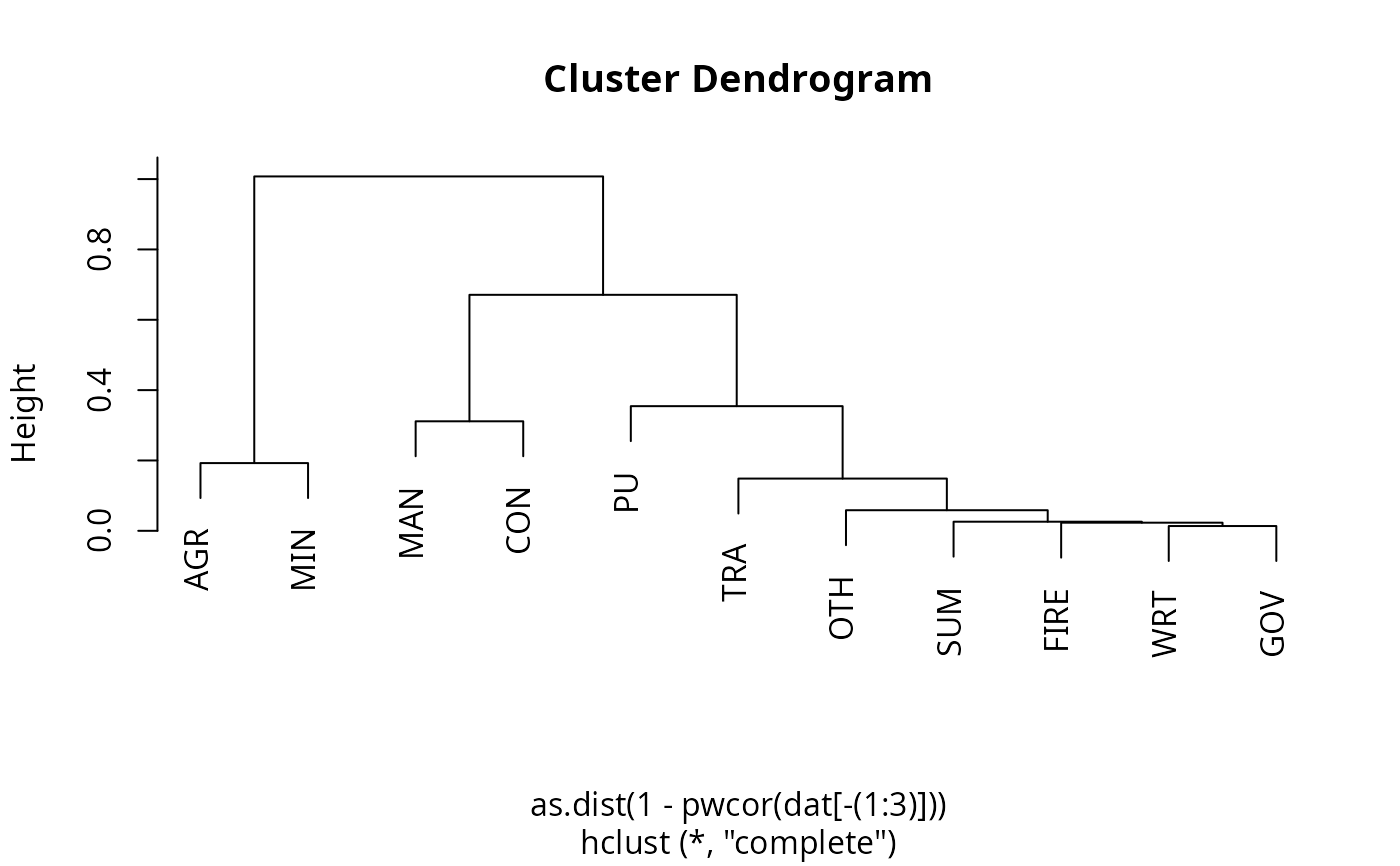
plot(hclust(as.dist(1-pwcor(dat[-(1:3)])))) # Using corrs. as distance metric to cluster sectors
 # List of panel-series matrices
psml <- psmat(fsubset(GGDC10S, Variable == "VA"), ~Country, ~Year, cols = 6:16, array = FALSE)
# Recombining with unlist2d() (effectively like reshapig the data)
head(unlist2d(psml, idcols = "Sector", row.names = "Country"))
#> Sector Country 1947 1948 1949 1950 1951 1952
#> 1 AGR ARG NA NA NA 5.887857e-07 9.165327e-07 9.964412e-07
#> 2 AGR BOL NA NA NA NA NA NA
#> 3 AGR BRA NA NA NA NA NA NA
#> 4 AGR BWA NA NA NA NA NA NA
#> 5 AGR CHL NA NA NA 1.488472e-02 1.757582e-02 2.508017e-02
#> 6 AGR CHN NA NA NA NA NA 3.459756e+04
#> 1953 1954 1955 1956 1957 1958
#> 1 1.482589e-06 1.396692e-06 1.574796e-06 2.001253e-06 2.644127e-06 3.741081e-06
#> 2 NA NA NA NA NA 1.824902e-01
#> 3 NA NA NA NA NA NA
#> 4 NA NA NA NA NA NA
#> 5 2.961345e-02 4.486172e-02 8.259973e-02 1.185127e-01 1.504810e-01 2.140646e-01
#> 6 3.813905e+04 3.955160e+04 4.247762e+04 4.478816e+04 4.338569e+04 4.498995e+04
#> 1959 1960 1961 1962 1963 1964
#> 1 8.395798e-06 1.028314e-05 9.868339e-06 1.342763e-05 1.902081e-05 2.947121e-05
#> 2 1.982476e-01 2.358937e-01 2.649170e-01 2.704523e-01 2.875517e-01 3.012666e-01
#> 3 NA NA NA NA NA NA
#> 4 NA NA NA NA NA 1.630154e+01
#> 5 2.719963e-01 3.261600e-01 3.488494e-01 3.757931e-01 5.672348e-01 9.097028e-01
#> 6 3.872425e+04 3.437559e+04 4.450564e+04 4.571641e+04 5.019623e+04 5.640140e+04
#> 1965 1966 1967 1968 1969 1970
#> 1 3.549257e-05 3.856346e-05 4.832476e-05 5.232561e-05 6.292321e-05 7.617020e-05
#> 2 3.247992e-01 3.456743e-01 3.558257e-01 3.999931e-01 3.887203e-01 4.120399e-01
#> 3 NA NA NA NA NA NA
#> 4 1.572700e+01 1.768066e+01 1.914591e+01 2.109957e+01 2.186221e+01 2.313327e+01
#> 5 1.264934e+00 1.593930e+00 2.112950e+00 2.342680e+00 3.904466e+00 5.466253e+00
#> 6 6.569400e+04 7.084984e+04 7.206060e+04 7.328146e+04 7.428033e+04 8.004155e+04
#> 1971 1972 1973 1974 1975 1976
#> 1 1.145865e-04 2.086401e-04 4.172802e-04 4.868269e-04 1.043201e-03 5.841923e-03
#> 2 4.411802e-01 4.819868e-01 7.372468e-01 1.290330e+00 1.431005e+00 1.603999e+00
#> 3 NA NA NA NA NA NA
#> 4 2.479488e+01 3.472939e+01 4.640244e+01 5.472259e+01 6.129982e+01 6.577234e+01
#> 5 7.808933e+00 1.327519e+01 6.247146e+01 4.299023e+02 1.918531e+03 8.926021e+03
#> 6 8.337115e+04 8.348214e+04 9.156398e+04 9.536780e+04 9.798103e+04 9.756735e+04
#> 1977 1978 1979 1980 1981 1982
#> 1 1.613484e-02 3.672066e-02 1.052937e-01 1.730322e-01 4.325805e-01 1.816838e+00
#> 2 1.804222e+00 2.032176e+00 2.380132e+00 3.563650e+00 3.760493e+00 1.736066e+01
#> 3 NA NA NA NA NA NA
#> 4 7.436659e+01 7.629591e+01 8.129461e+01 8.795954e+01 9.567683e+01 9.909699e+01
#> 5 2.325418e+04 3.045813e+04 4.613846e+04 6.387378e+04 6.852873e+04 6.216979e+04
#> 6 9.505502e+04 1.027535e+05 1.270192e+05 1.371593e+05 1.559463e+05 1.777401e+05
#> 1983 1984 1985 1986 1987 1988
#> 1 8.219029e+00 57.10062 350.3902 673.7874 1633.9430 8626.5202
#> 2 4.880016e+01 661.51794 711.0373 1773.3427 1401.7059 1700.2870
#> 3 NA NA NA NA NA NA
#> 4 8.918729e+01 90.76583 104.1834 116.1101 126.1952 235.0265
#> 5 7.431967e+04 111771.30832 168306.3369 251641.4921 342903.4319 431069.3741
#> 6 1.978387e+05 231608.94957 256439.6891 278869.0811 323304.0981 386536.2169
#> 1989 1990 1991 1992 1993 1994
#> 1 269.8437 4.843777e+03 1.051153e+04 1.175753e+04 12148.8501 13084.820
#> 2 1937.4890 2.371077e+03 2.973534e+03 3.170942e+03 3582.7410 4212.963
#> 3 NA 5.552811e-01 2.847801e+00 3.012148e+01 659.7625 21030.251
#> 4 252.3991 2.807167e+02 3.031157e+02 3.334364e+02 404.5488 425.400
#> 5 524494.6478 6.539881e+05 9.619029e+05 1.200560e+06 1240154.4872 1378480.745
#> 6 426592.3062 5.062000e+05 5.342200e+05 5.866600e+05 696376.2895 957269.475
#> 1995 1996 1997 1998 1999 2000
#> 1 13808.478 15269.958 15293.02 15702.922 12638.962 13300.482
#> 2 4789.906 5324.453 6212.54 5911.521 6384.542 6732.951
#> 3 35554.580 40958.485 44823.84 47844.729 50782.029 57241.000
#> 4 608.200 594.800 649.30 641.100 758.500 825.300
#> 5 1556231.378 1633764.436 1789913.98 1929978.863 1999335.365 2150247.820
#> 6 1213581.140 1401538.999 1444188.57 1481762.552 1477002.847 1494472.250
#> 2001 2002 2003 2004 2005 2006
#> 1 12275.652 31903.936 38824.561 43148.468 46330.594 50759.94
#> 2 7130.259 7343.263 8312.057 9275.858 9083.204 10034.96
#> 3 66819.000 84251.000 108619.000 115194.000 105163.000 111566.00
#> 4 830.600 834.800 1012.200 949.900 927.900 1210.70
#> 5 2031171.513 2302301.521 2607711.973 2662598.803 2930689.186 3113647.77
#> 6 1578126.905 1653701.966 1738171.770 2141273.404 2242000.000 2404000.00
#> 2007 2008 2009 2010 2011 2012 2013
#> 1 70101.51 93178.70 79362.85 132365.85 178745.30 NA NA
#> 2 10312.41 12603.33 13575.46 14325.14 16246.64 NA NA
#> 3 127267.00 152273.00 157232.00 171177.00 192654.00 NA NA
#> 4 1504.70 1887.50 2071.00 2717.30 NA NA NA
#> 5 3262339.12 3116984.64 3166792.56 3501045.92 3753294.19 NA NA
#> 6 2862700.00 3370200.00 3522600.00 4053360.00 4748621.06 NA NA
rm(l, dat, sdat, psml)
# List of panel-series matrices
psml <- psmat(fsubset(GGDC10S, Variable == "VA"), ~Country, ~Year, cols = 6:16, array = FALSE)
# Recombining with unlist2d() (effectively like reshapig the data)
head(unlist2d(psml, idcols = "Sector", row.names = "Country"))
#> Sector Country 1947 1948 1949 1950 1951 1952
#> 1 AGR ARG NA NA NA 5.887857e-07 9.165327e-07 9.964412e-07
#> 2 AGR BOL NA NA NA NA NA NA
#> 3 AGR BRA NA NA NA NA NA NA
#> 4 AGR BWA NA NA NA NA NA NA
#> 5 AGR CHL NA NA NA 1.488472e-02 1.757582e-02 2.508017e-02
#> 6 AGR CHN NA NA NA NA NA 3.459756e+04
#> 1953 1954 1955 1956 1957 1958
#> 1 1.482589e-06 1.396692e-06 1.574796e-06 2.001253e-06 2.644127e-06 3.741081e-06
#> 2 NA NA NA NA NA 1.824902e-01
#> 3 NA NA NA NA NA NA
#> 4 NA NA NA NA NA NA
#> 5 2.961345e-02 4.486172e-02 8.259973e-02 1.185127e-01 1.504810e-01 2.140646e-01
#> 6 3.813905e+04 3.955160e+04 4.247762e+04 4.478816e+04 4.338569e+04 4.498995e+04
#> 1959 1960 1961 1962 1963 1964
#> 1 8.395798e-06 1.028314e-05 9.868339e-06 1.342763e-05 1.902081e-05 2.947121e-05
#> 2 1.982476e-01 2.358937e-01 2.649170e-01 2.704523e-01 2.875517e-01 3.012666e-01
#> 3 NA NA NA NA NA NA
#> 4 NA NA NA NA NA 1.630154e+01
#> 5 2.719963e-01 3.261600e-01 3.488494e-01 3.757931e-01 5.672348e-01 9.097028e-01
#> 6 3.872425e+04 3.437559e+04 4.450564e+04 4.571641e+04 5.019623e+04 5.640140e+04
#> 1965 1966 1967 1968 1969 1970
#> 1 3.549257e-05 3.856346e-05 4.832476e-05 5.232561e-05 6.292321e-05 7.617020e-05
#> 2 3.247992e-01 3.456743e-01 3.558257e-01 3.999931e-01 3.887203e-01 4.120399e-01
#> 3 NA NA NA NA NA NA
#> 4 1.572700e+01 1.768066e+01 1.914591e+01 2.109957e+01 2.186221e+01 2.313327e+01
#> 5 1.264934e+00 1.593930e+00 2.112950e+00 2.342680e+00 3.904466e+00 5.466253e+00
#> 6 6.569400e+04 7.084984e+04 7.206060e+04 7.328146e+04 7.428033e+04 8.004155e+04
#> 1971 1972 1973 1974 1975 1976
#> 1 1.145865e-04 2.086401e-04 4.172802e-04 4.868269e-04 1.043201e-03 5.841923e-03
#> 2 4.411802e-01 4.819868e-01 7.372468e-01 1.290330e+00 1.431005e+00 1.603999e+00
#> 3 NA NA NA NA NA NA
#> 4 2.479488e+01 3.472939e+01 4.640244e+01 5.472259e+01 6.129982e+01 6.577234e+01
#> 5 7.808933e+00 1.327519e+01 6.247146e+01 4.299023e+02 1.918531e+03 8.926021e+03
#> 6 8.337115e+04 8.348214e+04 9.156398e+04 9.536780e+04 9.798103e+04 9.756735e+04
#> 1977 1978 1979 1980 1981 1982
#> 1 1.613484e-02 3.672066e-02 1.052937e-01 1.730322e-01 4.325805e-01 1.816838e+00
#> 2 1.804222e+00 2.032176e+00 2.380132e+00 3.563650e+00 3.760493e+00 1.736066e+01
#> 3 NA NA NA NA NA NA
#> 4 7.436659e+01 7.629591e+01 8.129461e+01 8.795954e+01 9.567683e+01 9.909699e+01
#> 5 2.325418e+04 3.045813e+04 4.613846e+04 6.387378e+04 6.852873e+04 6.216979e+04
#> 6 9.505502e+04 1.027535e+05 1.270192e+05 1.371593e+05 1.559463e+05 1.777401e+05
#> 1983 1984 1985 1986 1987 1988
#> 1 8.219029e+00 57.10062 350.3902 673.7874 1633.9430 8626.5202
#> 2 4.880016e+01 661.51794 711.0373 1773.3427 1401.7059 1700.2870
#> 3 NA NA NA NA NA NA
#> 4 8.918729e+01 90.76583 104.1834 116.1101 126.1952 235.0265
#> 5 7.431967e+04 111771.30832 168306.3369 251641.4921 342903.4319 431069.3741
#> 6 1.978387e+05 231608.94957 256439.6891 278869.0811 323304.0981 386536.2169
#> 1989 1990 1991 1992 1993 1994
#> 1 269.8437 4.843777e+03 1.051153e+04 1.175753e+04 12148.8501 13084.820
#> 2 1937.4890 2.371077e+03 2.973534e+03 3.170942e+03 3582.7410 4212.963
#> 3 NA 5.552811e-01 2.847801e+00 3.012148e+01 659.7625 21030.251
#> 4 252.3991 2.807167e+02 3.031157e+02 3.334364e+02 404.5488 425.400
#> 5 524494.6478 6.539881e+05 9.619029e+05 1.200560e+06 1240154.4872 1378480.745
#> 6 426592.3062 5.062000e+05 5.342200e+05 5.866600e+05 696376.2895 957269.475
#> 1995 1996 1997 1998 1999 2000
#> 1 13808.478 15269.958 15293.02 15702.922 12638.962 13300.482
#> 2 4789.906 5324.453 6212.54 5911.521 6384.542 6732.951
#> 3 35554.580 40958.485 44823.84 47844.729 50782.029 57241.000
#> 4 608.200 594.800 649.30 641.100 758.500 825.300
#> 5 1556231.378 1633764.436 1789913.98 1929978.863 1999335.365 2150247.820
#> 6 1213581.140 1401538.999 1444188.57 1481762.552 1477002.847 1494472.250
#> 2001 2002 2003 2004 2005 2006
#> 1 12275.652 31903.936 38824.561 43148.468 46330.594 50759.94
#> 2 7130.259 7343.263 8312.057 9275.858 9083.204 10034.96
#> 3 66819.000 84251.000 108619.000 115194.000 105163.000 111566.00
#> 4 830.600 834.800 1012.200 949.900 927.900 1210.70
#> 5 2031171.513 2302301.521 2607711.973 2662598.803 2930689.186 3113647.77
#> 6 1578126.905 1653701.966 1738171.770 2141273.404 2242000.000 2404000.00
#> 2007 2008 2009 2010 2011 2012 2013
#> 1 70101.51 93178.70 79362.85 132365.85 178745.30 NA NA
#> 2 10312.41 12603.33 13575.46 14325.14 16246.64 NA NA
#> 3 127267.00 152273.00 157232.00 171177.00 192654.00 NA NA
#> 4 1504.70 1887.50 2071.00 2717.30 NA NA NA
#> 5 3262339.12 3116984.64 3166792.56 3501045.92 3753294.19 NA NA
#> 6 2862700.00 3370200.00 3522600.00 4053360.00 4748621.06 NA NA
rm(l, dat, sdat, psml)