Solver for Ordinary Differential Equations; Assumes a Banded Jacobian

Solves a system of ordinary differential equations.

Assumes a banded Jacobian matrix, but does not rearrange the state variables (in contrast to ode.1D). Suitable for 1-D models that include transport only between adjacent layers and that model only one species.

ode.band(y, times, func, parms, nspec = NULL, dimens = NULL, 
  bandup = nspec, banddown = nspec, method = "lsode", names = NULL, 
  ...)

Arguments

y

the initial (state) values for the ODE system, a vector. If y has a name attribute, the names will be used to label the output matrix.

times

time sequence for which output is wanted; the first value of times must be the initial time.

func

either an R-function that computes the values of the derivatives in the ODE system (the model definition) at time t, or a character string giving the name of a compiled function in a dynamically loaded shared library.

If func is an R-function, it must be defined as: func <- function(t, y, parms, ...). t is the current time point in the integration, y is the current estimate of the variables in the ODE system. If the initial values y has a names attribute, the names will be available inside func. parms is a vector or list of parameters; ... (optional) are any other arguments passed to the function.

The return value of func should be a list, whose first element is a vector containing the derivatives of y with respect to time, and whose next elements are global values that are required at each point in times.The derivatives must be specified in the same order as the state variables y.

parms

parameters passed to func.

nspec

the number of *species* (components) in the model.

dimens

the number of boxes in the model. If NULL, then nspec should be specified.

bandup

the number of nonzero bands above the Jacobian diagonal.

banddown

the number of nonzero bands below the Jacobian diagonal.

method

the integrator to use, one of "vode", "lsode", "lsoda", "lsodar", "radau".

names

the names of the components; used for plotting.

...

additional arguments passed to the integrator.

Value

A matrix of class deSolve with up to as many rows as elements in times and as many columns as elements in y plus the number of "global" values returned in the second element of the return from func, plus an additional column (the first) for the time value. There will be one row for each element in times unless the integrator returns with an unrecoverable error. If y has a names attribute, it will be used to label the columns of the output value.

The output will have the attributes istate and rstate, two vectors with several elements. See the help for the selected integrator for details. the first element of istate returns the conditions under which the last call to the integrator returned. Normal is istate = 2. If verbose = TRUE, the settings of istate and rstate will be written to the screen.

Author

Karline Soetaert <karline.soetaert@nioz.nl>

Details

This is the method of choice for single-species 1-D reactive transport models.

For multi-species 1-D models, this method can only be used if the state variables are arranged per box, per species (e.g. A[1], B[1], A[2], B[2], A[3], B[3], ... for species A, B). By default, the model function will have the species arranged as A[1], A[2], A[3], ... B[1], B[2], B[3], ... in this case, use ode.1D.

See the selected integrator for the additional options.

Examples


## =======================================================================
## The Aphid model from Soetaert and Herman, 2009.
## A practical guide to ecological modelling.
## Using R as a simulation platform. Springer.
## =======================================================================

## 1-D diffusion model

## ================
## Model equations
## ================
Aphid <- function(t, APHIDS, parameters) {
  deltax  <- c (0.5*delx, rep(delx, numboxes-1), 0.5*delx)
  Flux    <- -D*diff(c(0, APHIDS, 0))/deltax
  dAPHIDS <- -diff(Flux)/delx + APHIDS*r

  list(dAPHIDS)   # the output
}
  
## ==================
## Model application
## ==================

## the model parameters:
D         <- 0.3    # m2/day  diffusion rate
r         <- 0.01   # /day    net growth rate
delx      <- 1      # m       thickness of boxes
numboxes  <- 60 

## distance of boxes on plant, m, 1 m intervals
Distance  <- seq(from = 0.5, by = delx, length.out = numboxes)

## Initial conditions, ind/m2
## aphids present only on two central boxes
APHIDS        <- rep(0, times = numboxes)
APHIDS[30:31] <- 1
state         <- c(APHIDS = APHIDS)      # initialise state variables 
                  
## RUNNING the model:
times <- seq(0, 200, by = 1)   # output wanted at these time intervals
out   <- ode.band(state, times, Aphid, parms = 0, 
                  nspec = 1, names = "Aphid")

## ================
## Plotting output
## ================
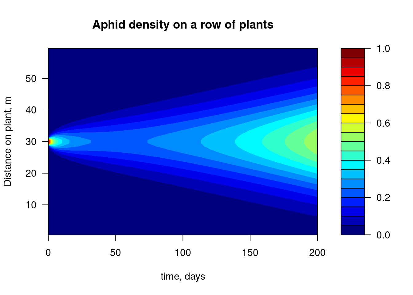
image(out, grid = Distance, method = "filled.contour", 
      xlab = "time, days", ylab = "Distance on plant, m",
      main = "Aphid density on a row of plants")


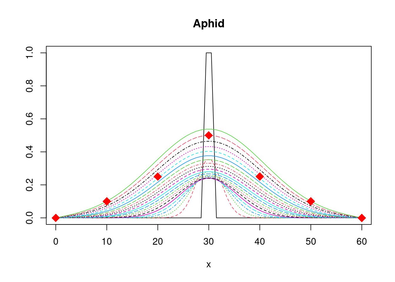
matplot.1D(out, grid = Distance, type = "l", 
   subset = time %in% seq(0, 200, by = 10))

# add an observed dataset to 1-D plot (make sure to use correct name):
data <- cbind(dist  = c(0,10, 20,  30,  40, 50, 60), 
              Aphid = c(0,0.1,0.25,0.5,0.25,0.1,0))

matplot.1D(out, grid = Distance, type = "l", 
   subset = time %in% seq(0, 200, by = 10), 
   obs = data, obspar = list(pch = 18, cex = 2, col="red"))

if (FALSE) { # \dontrun{
plot.1D(out, grid = Distance, type = "l")

} # }