Estimates OLS with any number of fixed-effects.
feols(
  fml,
  data,
  vcov,
  weights,
  offset,
  subset,
  split,
  fsplit,
  split.keep,
  split.drop,
  cluster,
  se,
  ssc,
  panel.id,
  fixef,
  fixef.rm = "none",
  fixef.tol = 1e-06,
  fixef.iter = 10000,
  fixef.algo = NULL,
  collin.tol = 1e-10,
  nthreads = getFixest_nthreads(),
  lean = FALSE,
  verbose = 0,
  warn = TRUE,
  notes = getFixest_notes(),
  only.coef = FALSE,
  data.save = FALSE,
  combine.quick,
  demeaned = FALSE,
  mem.clean = FALSE,
  only.env = FALSE,
  env,
  ...
)

feols.fit(
  y,
  X,
  fixef_df,
  vcov,
  offset,
  split,
  fsplit,
  split.keep,
  split.drop,
  cluster,
  se,
  ssc,
  weights,
  subset,
  fixef.rm = "perfect",
  fixef.tol = 1e-06,
  fixef.iter = 10000,
  fixef.algo = NULL,
  collin.tol = 1e-10,
  nthreads = getFixest_nthreads(),
  lean = FALSE,
  warn = TRUE,
  notes = getFixest_notes(),
  mem.clean = FALSE,
  verbose = 0,
  only.env = FALSE,
  only.coef = FALSE,
  env,
  ...
)
Arguments
- fml
A formula representing the relation to be estimated. For example:
fml = z~x+y. To include fixed-effects, insert them in this formula using a pipe: e.g.fml = z~x+y | fe_1+fe_2. You can combine two fixed-effects with^: e.g.fml = z~x+y|fe_1^fe_2, see details. You can also use variables with varying slopes using square brackets: e.g. infml = z~y|fe_1[x] + fe_2, see details. To add IVs, insert the endogenous vars./instruments after a pipe, like iny ~ x | x_endo1 + x_endo2 ~ x_inst1 + x_inst2. Note that it should always be the last element, see details. Multiple estimations can be performed at once: for multiple dep. vars, wrap them inc(): exc(y1, y2). For multiple indep. vars, use the stepwise functions: exx1 + csw(x2, x3). The formulafml = c(y1, y2) ~ x1 + cw0(x2, x3)leads to 6 estimation, see details. Square brackets starting with a dot can be used to call global variables:y.[i] ~ x.[1:2]will lead toy3 ~ x1 + x2ifiis equal to 3 in the current environment (see details inxpd).- data
A data.frame containing the necessary variables to run the model. The variables of the non-linear right hand side of the formula are identified with this
data.framenames. Can also be a matrix.- vcov
Versatile argument to specify the VCOV. In general, it is either a character scalar equal to a VCOV type, either a formula of the form:
vcov_type ~ variables. The VCOV types implemented are: "iid", "hetero" (or "HC1"), "cluster", "twoway", "NW" (or "newey_west"), "DK" (or "driscoll_kraay"), and "conley". It also accepts object fromvcov_cluster,vcov_NW,NW,vcov_DK,DK,vcov_conleyandconley. It also accepts covariance matrices computed externally. Finally it accepts functions to compute the covariances. See thevcovdocumentation in the vignette.- weights
A formula or a numeric vector. Each observation can be weighted, the weights must be greater than 0. If equal to a formula, it should be one-sided: for example
~ var_weight.- offset
A formula or a numeric vector. An offset can be added to the estimation. If equal to a formula, it should be of the form (for example)
~0.5*x**2. This offset is linearly added to the elements of the main formula 'fml'.- subset
A vector (logical or numeric) or a one-sided formula. If provided, then the estimation will be performed only on the observations defined by this argument.
- split
A one sided formula representing a variable (eg
split = ~var) or a vector. If provided, the sample is split according to the variable and one estimation is performed for each value of that variable. If you also want to include the estimation for the full sample, use the argumentfsplitinstead. You can use the special operators%keep%and%drop%to select only a subset of values for which to split the sample. E.g.split = ~var %keep% c("v1", "v2")will split the sample only according to the valuesv1andv2of the variablevar; it is equivalent to supplying the argumentsplit.keep = c("v1", "v2"). By default there is partial matching on each value, you can trigger a regular expression evaluation by adding a'@'first, as in:~var %drop% "@^v[12]"which will drop values starting with"v1"or"v2"(of course you need to know regexes!).- fsplit
A one sided formula representing a variable (eg
fsplit = ~var) or a vector. If provided, the sample is split according to the variable and one estimation is performed for each value of that variable. This argument is the same assplitbut also includes the full sample as the first estimation. You can use the special operators%keep%and%drop%to select only a subset of values for which to split the sample. E.g.fsplit = ~var %keep% c("v1", "v2")will split the sample only according to the valuesv1andv2of the variablevar; it is equivalent to supplying the argumentsplit.keep = c("v1", "v2"). By default there is partial matching on each value, you can trigger a regular expression evaluation by adding an'@'first, as in:~var %drop% "@^v[12]"which will drop values starting with"v1"or"v2"(of course you need to know regexes!).- split.keep
A character vector. Only used when
split, orfsplit, is supplied. If provided, then the sample will be split only on the values ofsplit.keep. The values insplit.keepwill be partially matched to the values ofsplit. To enable regular expressions, you need to add an'@'first. For examplesplit.keep = c("v1", "@other|var")will keep only the value insplitpartially matched by"v1"or the values containing"other"or"var".- split.drop
A character vector. Only used when
split, orfsplit, is supplied. If provided, then the sample will be split only on the values that are not insplit.drop. The values insplit.dropwill be partially matched to the values ofsplit. To enable regular expressions, you need to add an'@'first. For examplesplit.drop = c("v1", "@other|var")will drop only the value insplitpartially matched by"v1"or the values containing"other"or"var".- cluster
Tells how to cluster the standard-errors (if clustering is requested). Can be either a list of vectors, a character vector of variable names, a formula or an integer vector. Assume we want to perform 2-way clustering over
var1andvar2contained in the data.framebaseused for the estimation. All the followingclusterarguments are valid and do the same thing:cluster = base[, c("var1", "var2")],cluster = c("var1", "var2"),cluster = ~var1+var2. If the two variables were used as fixed-effects in the estimation, you can leave it blank withvcov = "twoway"(assumingvar1[resp.var2] was the 1st [resp. 2nd] fixed-effect). You can interact two variables using^with the following syntax:cluster = ~var1^var2orcluster = "var1^var2".- se
Character scalar. Which kind of standard error should be computed: “standard”, “hetero”, “cluster”, “twoway”, “threeway” or “fourway”? By default if there are clusters in the estimation:
se = "cluster", otherwisese = "iid". Note that this argument is deprecated, you should usevcovinstead.- ssc
An object of class
ssc.typeobtained with the functionssc. Represents how the degree of freedom correction should be done.You must use the functionsscfor this argument. The arguments and defaults of the functionsscare:adj = TRUE,fixef.K="nested",cluster.adj = TRUE,cluster.df = "min",t.df = "min",fixef.force_exact=FALSE). See the help of the functionsscfor details.- panel.id
The panel identifiers. Can either be: i) a one sided formula (e.g.
panel.id = ~id+time), ii) a character vector of length 2 (e.g.panel.id=c('id', 'time'), or iii) a character scalar of two variables separated by a comma (e.g.panel.id='id,time'). Note that you can combine variables with^only inside formulas (see the dedicated section infeols).- fixef
Character vector. The names of variables to be used as fixed-effects. These variables should contain the identifier of each observation (e.g., think of it as a panel identifier). Note that the recommended way to include fixed-effects is to insert them directly in the formula.
- fixef.rm
Can be equal to "perfect" (default), "singleton", "both" or "none". Controls which observations are to be removed. If "perfect", then observations having a fixed-effect with perfect fit (e.g. only 0 outcomes in Poisson estimations) will be removed. If "singleton", all observations for which a fixed-effect appears only once will be removed. Note, importantly, that singletons are removed in just one pass, there is no recursivity implemented. The meaning of "both" and "none" is direct.
- fixef.tol
Precision used to obtain the fixed-effects. Defaults to
1e-5. It corresponds to the maximum absolute difference allowed between two coefficients of successive iterations. Argumentfixef.tolcannot be lower than10000*.Machine$double.eps. Note that this parameter is dynamically controlled by the algorithm.- fixef.iter
Maximum number of iterations in fixed-effects algorithm (only in use for 2+ fixed-effects). Default is 10000.
- fixef.algo
NULL(default) or an object of classdemeaning_algoobtained with the functiondemeaning_algo. IfNULL, it falls to the defaults ofdemeaning_algo. This arguments controls the settings of the demeaning algorithm. Only play with it if the convergence is slow, i.e. look at the slot$iterations, and if any is over 50, it may be worth playing around with it. Please read the documentation of the functiondemeaning_algo. Be aware that there is no clear guidance on how to change the settings, it's more a matter of try-and-see.- collin.tol
Numeric scalar, default is
1e-10. Threshold deciding when variables should be considered collinear and subsequently removed from the estimation. Higher values means more variables will be removed (if there is presence of collinearity). One signal of presence of collinearity is t-stats that are extremely low (for instance when t-stats < 1e-3).- nthreads
The number of threads. Can be: a) an integer lower than, or equal to, the maximum number of threads; b) 0: meaning all available threads will be used; c) a number strictly between 0 and 1 which represents the fraction of all threads to use. The default is to use 50% of all threads. You can set permanently the number of threads used within this package using the function
setFixest_nthreads.- lean
Logical, default is
FALSE. IfTRUEthen all large objects are removed from the returned result: this will save memory but will block the possibility to use many methods. It is recommended to use the argumentsseorclusterto obtain the appropriate standard-errors at estimation time, since obtaining different SEs won't be possible afterwards.- verbose
Integer. Higher values give more information. In particular, it can detail the number of iterations in the demeaning algorithm (the first number is the left-hand-side, the other numbers are the right-hand-side variables).
- warn
Logical, default is
TRUE. Whether warnings should be displayed (concerns warnings relating to convergence state).- notes
Logical. By default, two notes are displayed: when NAs are removed (to show additional information) and when some observations are removed because of collinearity. To avoid displaying these messages, you can set
notes = FALSE. You can remove these messages permanently by usingsetFixest_notes(FALSE).- only.coef
Logical, default is
FALSE. IfTRUE, then only the estimated coefficients are returned. Note that the length of the vector returned is always the length of the number of coefficients to be estimated: this means that the variables found to be collinear are returned with an NA value.- data.save
Logical scalar, default is
FALSE. IfTRUE, the data used for the estimation is saved within the returned object. Hence later calls to predict(), vcov(), etc..., will be consistent even if the original data has been modified in the meantime. This is especially useful for estimations within loops, where the data changes at each iteration, such that postprocessing can be done outside the loop without issue.- combine.quick
Logical. When you combine different variables to transform them into a single fixed-effects you can do e.g.
y ~ x | paste(var1, var2). The algorithm provides a shorthand to do the same operation:y ~ x | var1^var2. Because pasting variables is a costly operation, the internal algorithm may use a numerical trick to hasten the process. The cost of doing so is that you lose the labels. If you are interested in getting the value of the fixed-effects coefficients after the estimation, you should usecombine.quick = FALSE. By default it is equal toFALSEif the number of observations is lower than 50,000, and toTRUEotherwise.- demeaned
Logical, default is
FALSE. Only used in the presence of fixed-effects: should the centered variables be returned? IfTRUE, it creates the itemsy_demeanedandX_demeaned.- mem.clean
Logical, default is
FALSE. Only to be used if the data set is large compared to the available RAM. IfTRUEthen intermediary objects are removed as much as possible andgcis run before each substantial C++ section in the internal code to avoid memory issues.- only.env
(Advanced users.) Logical, default is
FALSE. IfTRUE, then only the environment used to make the estimation is returned.- env
(Advanced users.) A
fixestenvironment created by afixestestimation withonly.env = TRUE. Default is missing. If provided, the data from this environment will be used to perform the estimation.- ...
Not currently used.
- y
Numeric vector/matrix/data.frame of the dependent variable(s). Multiple dependent variables will return a
fixest_multiobject.- X
Numeric matrix of the regressors.
- fixef_df
Matrix/data.frame of the fixed-effects.
Value
A fixest object. Note that fixest objects contain many elements and most of them are
for internal use, they are presented here only for information. To access them, it is safer
to use the user-level methods (e.g. vcov.fixest, resid.fixest, etc) or functions
(like for instance fitstat to access any fit statistic).
- nobs
The number of observations.
- fml
The linear formula of the call.
- call
The call of the function.
- method
The method used to estimate the model.
- data
The original data set used when calling the function. Only available when the estimation was called with
data.save = TRUE- fml_all
A list containing different parts of the formula. Always contain the linear formula. Then depending on the cases:
fixef: the fixed-effects,iv: the IV part of the formula.- fixef_vars
The names of each fixed-effect dimension.
- fixef_id
The list (of length the number of fixed-effects) of the fixed-effects identifiers for each observation.
- fixef_sizes
The size of each fixed-effect (i.e. the number of unique identifierfor each fixed-effect dimension).
- coefficients
The named vector of estimated coefficients.
- multicol
Logical, if multicollinearity was found.
- coeftable
The table of the coefficients with their standard errors, z-values and p-values.
- loglik
The loglikelihood.
- ssr_null
Sum of the squared residuals of the null model (containing only with the intercept).
- ssr_fe_only
Sum of the squared residuals of the model estimated with fixed-effects only.
- ll_null
The log-likelihood of the null model (containing only with the intercept).
- ll_fe_only
The log-likelihood of the model estimated with fixed-effects only.
- fitted.values
The fitted values.
- linear.predictors
The linear predictors.
- residuals
The residuals (y minus the fitted values).
- sq.cor
Squared correlation between the dependent variable and the expected predictor (i.e. fitted.values) obtained by the estimation.
- hessian
The Hessian of the parameters.
- cov.iid
The variance-covariance matrix of the parameters.
- se
The standard-error of the parameters.
- scores
The matrix of the scores (first derivative for each observation).
- residuals
The difference between the dependent variable and the expected predictor.
- sumFE
The sum of the fixed-effects coefficients for each observation.
- offset
(When relevant.) The offset formula.
- weights
(When relevant.) The weights formula.
- obs_selection
(When relevant.) List containing vectors of integers. It represents the sequential selection of observation vis a vis the original data set.
- collin.var
(When relevant.) Vector containing the variables removed because of collinearity.
- collin.coef
(When relevant.) Vector of coefficients, where the values of the variables removed because of collinearity are NA.
- collin.min_norm
The minimal diagonal value of the Cholesky decomposition. Small values indicate possible presence collinearity.
- y_demeaned
Only when
demeaned = TRUE: the centered dependent variable.- X_demeaned
Only when
demeaned = TRUE: the centered explanatory variable.
Details
The method used to demean each variable along the fixed-effects is based on Berge (2018), since this is the same problem to solve as for the Gaussian case in a ML setup.
Combining the fixed-effects
You can combine two variables to make it a new fixed-effect using ^.
The syntax is as follows: fe_1^fe_2. Here you created a new variable which is the combination
of the two variables fe_1 and fe_2. This is identical to doing paste0(fe_1, "_", fe_2)
but more convenient.
Note that pasting is a costly operation, especially for large data sets.
Thus, the internal algorithm uses a numerical trick which is fast, but the drawback is
that the identity of each observation is lost (i.e. they are now equal to a meaningless
number instead of being equal to paste0(fe_1, "_", fe_2)). These “identities”
are useful only if you're interested in the value of the fixed-effects (that you can
extract with fixef.fixest). If you're only interested in coefficients of the variables,
it doesn't matter. Anyway, you can use combine.quick = FALSE to tell the internal
algorithm to use paste instead of the numerical trick. By default, the numerical
trick is performed only for large data sets.
Varying slopes
You can add variables with varying slopes in the fixed-effect part of the formula.
The syntax is as follows: fixef_var[var1, var2]. Here the variables var1 and var2 will
be with varying slopes (one slope per value in fixef_var) and the fixed-effect
fixef_var will also be added.
To add only the variables with varying slopes and not the fixed-effect,
use double square brackets: fixef_var[[var1, var2]].
In other words:
fixef_var[var1, var2]is equivalent tofixef_var + fixef_var[[var1]] + fixef_var[[var2]]fixef_var[[var1, var2]]is equivalent tofixef_var[[var1]] + fixef_var[[var2]]
In general, for convergence reasons, it is recommended to always add the fixed-effect and avoid using only the variable with varying slope (i.e. use single square brackets).
Lagging variables
To use leads/lags of variables in the estimation, you can: i) either provide the argument
panel.id, ii) either set your data set as a panel with the function
panel, f and d.
You can provide several leads/lags/differences at once: e.g. if your formula is equal to
f(y) ~ l(x, -1:1), it means that the dependent variable is equal to the lead of y,
and you will have as explanatory variables the lead of x1, x1 and the lag of x1.
See the examples in function l for more details.
Interactions
You can interact a numeric variable with a "factor-like" variable by using
i(factor_var, continuous_var, ref), where continuous_var will be interacted with
each value of factor_var and the argument ref is a value of factor_var
taken as a reference (optional).
Using this specific way to create interactions leads to a different display of the
interacted values in etable. See examples.
It is important to note that if you do not care about the standard-errors of
the interactions, then you can add interactions in the fixed-effects part of the formula,
it will be incomparably faster (using the syntax factor_var[continuous_var], as explained
in the section “Varying slopes”).
The function i has in fact more arguments, please see details in its associated help page.
On standard-errors
Standard-errors can be computed in different ways, you can use the arguments se and ssc
in summary.fixest to define how to compute them. By default, in the presence
of fixed-effects, standard-errors are automatically clustered.
The following vignette: On standard-errors describes in details how the standard-errors are computed in
fixest and how you can replicate standard-errors from other software.
You can use the functions setFixest_vcov and setFixest_ssc to
permanently set the way the standard-errors are computed.
Instrumental variables
To estimate two stage least square regressions, insert the relationship between the endogenous regressor(s) and the instruments in a formula, after a pipe.
For example, fml = y ~ x1 | x_endo ~ x_inst will use the variables x1 and x_inst in
the first stage to explain x_endo. Then will use the fitted value of x_endo
(which will be named fit_x_endo) and x1 to explain y.
To include several endogenous regressors, just use "+",
like in: fml = y ~ x1 | x_endo1 + x_end2 ~ x_inst1 + x_inst2.
Of course you can still add the fixed-effects, but the IV formula must always come last,
like in fml = y ~ x1 | fe1 + fe2 | x_endo ~ x_inst.
If you want to estimate a model without exogenous variables, use "1" as a
placeholder: e.g. fml = y ~ 1 | x_endo ~ x_inst.
By default, the second stage regression is returned. You can access the first stage(s)
regressions either directly in the slot iv_first_stage (not recommended),
or using the argument stage = 1 from the function summary.fixest.
For example summary(iv_est, stage = 1) will give the first stage(s).
Note that using summary you can display both the second and first stages at
the same time using, e.g., stage = 1:2 (using 2:1 would reverse the order).
Multiple estimations
Multiple estimations can be performed at once, they just have to be specified in the formula.
Multiple estimations yield a fixest_multi object which is ‘kind of’ a list of
all the results but includes specific methods to access the results in a handy way.
Please have a look at the dedicated vignette:
Multiple estimations.
To include multiple dependent variables, wrap them in c() (list() also works).
For instance fml = c(y1, y2) ~ x1 would estimate the model fml = y1 ~ x1 and
then the model fml = y2 ~ x1.
To include multiple independent variables, you need to use the stepwise functions.
There are 4 stepwise functions: sw, sw0, csw, csw0, and mvsw. Of course sw
stands for stepwise, and csw for cumulative stepwise. Finally mvsw is a bit special,
it stands for multiverse stepwise. Let's explain that.
Assume you have the following formula: fml = y ~ x1 + sw(x2, x3).
The stepwise function sw will estimate the following two models: y ~ x1 + x2 and
y ~ x1 + x3. That is, each element in sw() is sequentially, and separately,
added to the formula. Would have you used sw0 in lieu of sw, then the model
y ~ x1 would also have been estimated. The 0 in the name means that the model
without any stepwise element also needs to be estimated.
The prefix c means cumulative: each stepwise element is added to the next. That is,
fml = y ~ x1 + csw(x2, x3) would lead to the following models y ~ x1 + x2 and
y ~ x1 + x2 + x3. The 0 has the same meaning and would also lead to the model without
the stepwise elements to be estimated: in other words, fml = y ~ x1 + csw0(x2, x3)
leads to the following three models: y ~ x1, y ~ x1 + x2 and y ~ x1 + x2 + x3.
Finally mvsw will add, in a stepwise fashion all possible combinations of the variables
in its arguments. For example mvsw(x1, x2, x3) is equivalent to
sw0(x1, x2, x3, x1 + x2, x1 + x3, x2 + x3, x1 + x2 + x3). The number of models
to estimate grows at a factorial rate: so be cautious!
Multiple independent variables can be combined with multiple dependent variables, as in
fml = c(y1, y2) ~ cw(x1, x2, x3) which would lead to 6 estimations. Multiple
estimations can also be combined to split samples (with the arguments split, fsplit).
You can also add fixed-effects in a stepwise fashion. Note that you cannot perform
stepwise estimations on the IV part of the formula (feols only).
If NAs are present in the sample, to avoid too many messages, only NA removal concerning the variables common to all estimations is reported.
A note on performance. The feature of multiple estimations has been highly optimized for
feols, in particular in the presence of fixed-effects. It is faster to estimate
multiple models using the formula rather than with a loop. For non-feols models using
the formula is roughly similar to using a loop performance-wise.
Tricks to estimate multiple LHS
To use multiple dependent variables in fixest estimations, you need to include them
in a vector: like in c(y1, y2, y3).
First, if names are stored in a vector, they can readily be inserted in a formula to
perform multiple estimations using the dot square bracket operator. For instance if
my_lhs = c("y1", "y2"), calling fixest with, say feols(.[my_lhs] ~ x1, etc) is
equivalent to using feols(c(y1, y2) ~ x1, etc). Beware that this is a special feature
unique to the left-hand-side of fixest estimations (the default behavior of the DSB
operator is to aggregate with sums, see xpd).
Second, you can use a regular expression to grep the left-hand-sides on the fly. When the
..("regex") feature is used naked on the LHS, the variables grepped are inserted into
c(). For example ..("Pe") ~ Sepal.Length, iris is equivalent to
c(Petal.Length, Petal.Width) ~ Sepal.Length, iris. Beware that this is a
special feature unique to the left-hand-side of fixest estimations
(the default behavior of ..("regex") is to aggregate with sums, see xpd).
Argument sliding
When the data set has been set up globally using
setFixest_estimation(data = data_set), the argument vcov can be used implicitly.
This means that calls such as feols(y ~ x, "HC1"), or feols(y ~ x, ~id), are valid:
i) the data is automatically deduced from the global settings, and ii) the vcov
is deduced to be the second argument.
Piping
Although the argument 'data' is placed in second position, the data can be piped to the
estimation functions. For example, with R >= 4.1, mtcars |> feols(mpg ~ cyl) works as
feols(mpg ~ cyl, mtcars).
Dot square bracket operator in formulas
In a formula, the dot square bracket (DSB) operator can: i) create manifold variables at once, or ii) capture values from the current environment and put them verbatim in the formula.
Say you want to include the variables x1 to x3 in your formula. You can use
xpd(y ~ x.[1:3]) and you'll get y ~ x1 + x2 + x3.
To summon values from the environment, simply put the variable in square brackets. For example:
for(i in 1:3) xpd(y.[i] ~ x) will create the formulas y1 ~ x to y3 ~ x depending on the
value of i.
You can include a full variable from the environment in the same way:
for(y in c("a", "b")) xpd(.[y] ~ x) will create the two formulas a ~ x and b ~ x.
The DSB can even be used within variable names, but then the variable must be nested in
character form. For example y ~ .["x.[1:2]_sq"] will create y ~ x1_sq + x2_sq. Using the
character form is important to avoid a formula parsing error. Double quotes must be used. Note
that the character string that is nested will be parsed with the function dsb, and thus it
will return a vector.
By default, the DSB operator expands vectors into sums. You can add a comma, like in .[, x],
to expand with commas–the content can then be used within functions. For instance:
c(x.[, 1:2]) will create c(x1, x2) (and not c(x1 + x2)).
In all fixest estimations, this special parsing is enabled, so you don't need to use xpd.
One-sided formulas can be expanded with the DSB operator: let x = ~sepal + petal, then
xpd(y ~ .[x]) leads to color ~ sepal + petal.
You can even use multiple square brackets within a single variable, but then the use of nesting
is required. For example, the following xpd(y ~ .[".[letters[1:2]]_.[1:2]"]) will create
y ~ a_1 + b_2. Remember that the nested character string is parsed with dsb,
which explains this behavior.
When the element to be expanded i) is equal to the empty string or, ii) is of length 0, it is
replaced with a neutral element, namely 1. For example, x = "" ; xpd(y ~ .[x]) leads to
y ~ 1.
References
Berge, Laurent, 2018, "Efficient estimation of maximum likelihood models with multiple fixed-effects: the R package FENmlm." CREA Discussion Papers, 13 ().
For models with multiple fixed-effects:
Gaure, Simen, 2013, "OLS with multiple high dimensional category variables", Computational Statistics & Data Analysis 66 pp. 8–18
See also
See also summary.fixest to see the results with the appropriate standard-errors,
fixef.fixest to extract the fixed-effects coefficients, and the function etable
to visualize the results of multiple estimations. For plotting coefficients: see coefplot.
And other estimation methods: femlm, feglm, fepois, fenegbin, feNmlm.
Examples
#
# Basic estimation
#
res = feols(Sepal.Length ~ Sepal.Width + Petal.Length, iris)
# You can specify clustered standard-errors in summary:
summary(res, cluster = ~Species)
#> OLS estimation, Dep. Var.: Sepal.Length
#> Observations: 150
#> Standard-errors: Clustered (Species)
#> Estimate Std. Error t value Pr(>|t|)
#> (Intercept) 2.249140 0.162626 13.8302 0.00518747 **
#> Sepal.Width 0.595525 0.051733 11.5115 0.00746202 **
#> Petal.Length 0.471920 0.006873 68.6673 0.00021201 ***
#> ---
#> Signif. codes: 0 '***' 0.001 '**' 0.01 '*' 0.05 '.' 0.1 ' ' 1
#> RMSE: 0.329937 Adj. R2: 0.838003
#
# Just one set of fixed-effects:
#
res = feols(Sepal.Length ~ Sepal.Width + Petal.Length | Species, iris)
# By default, the SEs are clustered according to the first fixed-effect
summary(res)
#> OLS estimation, Dep. Var.: Sepal.Length
#> Observations: 150
#> Fixed-effects: Species: 3
#> Standard-errors: Clustered (Species)
#> Estimate Std. Error t value Pr(>|t|)
#> Sepal.Width 0.432217 0.161308 2.67945 0.115623
#> Petal.Length 0.775629 0.126546 6.12925 0.025601 *
#> ---
#> Signif. codes: 0 '***' 0.001 '**' 0.01 '*' 0.05 '.' 0.1 ' ' 1
#> RMSE: 0.305129 Adj. R2: 0.859538
#> Within R2: 0.641507
#
# Varying slopes:
#
res = feols(Sepal.Length ~ Petal.Length | Species[Sepal.Width], iris)
summary(res)
#> OLS estimation, Dep. Var.: Sepal.Length
#> Observations: 150
#> Fixed-effects: Species: 3
#> Varying slopes: Sepal.Width (Species): 3
#> Standard-errors: Clustered (Species)
#> Estimate Std. Error t value Pr(>|t|)
#> Petal.Length 0.822045 0.10061 8.1706 0.014651 *
#> ---
#> Signif. codes: 0 '***' 0.001 '**' 0.01 '*' 0.05 '.' 0.1 ' ' 1
#> RMSE: 0.298903 Adj. R2: 0.863326
#> Within R2: 0.518738
#
# Combining the FEs:
#
base = iris
base$fe_2 = rep(1:10, 15)
res_comb = feols(Sepal.Length ~ Petal.Length | Species^fe_2, base)
summary(res_comb)
#> OLS estimation, Dep. Var.: Sepal.Length
#> Observations: 150
#> Fixed-effects: Species^fe_2: 30
#> Standard-errors: Clustered (Species^fe_2)
#> Estimate Std. Error t value Pr(>|t|)
#> Petal.Length 0.875613 0.062395 14.0334 1.8483e-14 ***
#> ---
#> Signif. codes: 0 '***' 0.001 '**' 0.01 '*' 0.05 '.' 0.1 ' ' 1
#> RMSE: 0.309865 Adj. R2: 0.823494
#> Within R2: 0.548794
fixef(res_comb)[[1]]
#> setosa_1 setosa_10 setosa_2 setosa_3 setosa_4
#> 3.826581 3.646581 3.661605 3.601703 3.621605
#> setosa_5 setosa_6 setosa_7 setosa_8 setosa_9
#> 3.736532 3.884093 3.859118 3.699118 3.721605
#> versicolor_1 versicolor_10 versicolor_2 versicolor_3 versicolor_4
#> 2.067402 2.142623 2.322426 2.359841 1.922328
#> versicolor_5 versicolor_6 versicolor_7 versicolor_8 versicolor_9
#> 2.187402 2.287304 2.209694 2.284914 2.274963
#> virginica_1 virginica_10 virginica_2 virginica_3 virginica_4
#> 1.769007 1.841642 1.826716 1.716471 1.639252
#> virginica_5 virginica_6 virginica_7 virginica_8 virginica_9
#> 1.474081 2.006422 1.591887 1.791495 1.609007
#
# Using leads/lags:
#
data(base_did)
# We need to set up the panel with the arg. panel.id
est1 = feols(y ~ l(x1, 0:1), base_did, panel.id = ~id+period)
#> NOTE: 108 observations removed because of NA values (RHS: 108).
est2 = feols(f(y) ~ l(x1, -1:1), base_did, panel.id = ~id+period)
#> NOTE: 216 observations removed because of NA values (LHS: 108, RHS: 216).
etable(est1, est2, order = "f", drop="Int")
#> est1 est2
#> Dependent Var.: y f(y,1)
#>
#> f(x1,1) 0.9940*** (0.0542)
#> Constant 2.235*** (0.2032) 2.464*** (0.2233)
#> x1 0.9948*** (0.0487) 0.0081 (0.0592)
#> l(x1,1) 0.0410 (0.0558) 0.0157 (0.0640)
#> _______________ __________________ __________________
#> S.E.: Clustered by: id by: id
#> Observations 972 864
#> R2 0.26558 0.25697
#> Adj. R2 0.26406 0.25438
#> ---
#> Signif. codes: 0 '***' 0.001 '**' 0.01 '*' 0.05 '.' 0.1 ' ' 1
#
# Using interactions:
#
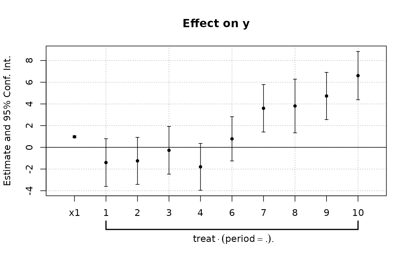
data(base_did)
# We interact the variable 'period' with the variable 'treat'
est_did = feols(y ~ x1 + i(period, treat, 5) | id+period, base_did)
# Now we can plot the result of the interaction with coefplot
coefplot(est_did)
 # You have many more example in coefplot help
#
# Instrumental variables
#
# To estimate Two stage least squares,
# insert a formula describing the endo. vars./instr. relation after a pipe:
base = iris
names(base) = c("y", "x1", "x2", "x3", "fe1")
base$x_inst1 = 0.2 * base$x1 + 0.7 * base$x2 + rpois(150, 2)
base$x_inst2 = 0.2 * base$x2 + 0.7 * base$x3 + rpois(150, 3)
base$x_endo1 = 0.5 * base$y + 0.5 * base$x3 + rnorm(150, sd = 2)
base$x_endo2 = 1.5 * base$y + 0.5 * base$x3 + 3 * base$x_inst1 + rnorm(150, sd = 5)
# Using 2 controls, 1 endogenous var. and 1 instrument
res_iv = feols(y ~ x1 + x2 | x_endo1 ~ x_inst1, base)
# The second stage is the default
summary(res_iv)
#> TSLS estimation - Dep. Var.: y
#> Endo. : x_endo1
#> Instr. : x_inst1
#> Second stage: Dep. Var.: y
#> Observations: 150
#> Standard-errors: IID
#> Estimate Std. Error t value Pr(>|t|)
#> (Intercept) 2.121500 0.491863 4.313190 2.9480e-05 ***
#> fit_x_endo1 0.045847 0.152955 0.299740 7.6480e-01
#> x1 0.607079 0.078881 7.696098 1.9324e-12 ***
#> x2 0.452870 0.065787 6.883914 1.6001e-10 ***
#> ---
#> Signif. codes: 0 '***' 0.001 '**' 0.01 '*' 0.05 '.' 0.1 ' ' 1
#> RMSE: 0.32641 Adj. R2: 0.840362
#> F-test (1st stage), x_endo1: stat = 1.23339, p = 0.268574, on 1 and 146 DoF.
#> Wu-Hausman: stat = 0.01126, p = 0.91564 , on 1 and 145 DoF.
# To show the first stage:
summary(res_iv, stage = 1)
#> TSLS estimation - Dep. Var.: x_endo1
#> Endo. : x_endo1
#> Instr. : x_inst1
#> First stage: Dep. Var.: x_endo1
#> Observations: 150
#> Standard-errors: IID
#> Estimate Std. Error t value Pr(>|t|)
#> (Intercept) 2.909227 1.453480 2.001560 0.04718500 *
#> x_inst1 -0.134265 0.120896 -1.110583 0.26857365
#> x1 -0.192889 0.408628 -0.472039 0.63760357
#> x2 0.517817 0.135988 3.807808 0.00020585 ***
#> ---
#> Signif. codes: 0 '***' 0.001 '**' 0.01 '*' 0.05 '.' 0.1 ' ' 1
#> RMSE: 1.92154 Adj. R2: 0.131456
#> F-test (1st stage): stat = 1.23339, p = 0.268574, on 1 and 146 DoF.
# To show both the first and second stages:
summary(res_iv, stage = 1:2)
#> IV: First stage: x_endo1
#> TSLS estimation - Dep. Var.: x_endo1
#> Endo. : x_endo1
#> Instr. : x_inst1
#> First stage: Dep. Var.: x_endo1
#> Observations: 150
#> Standard-errors: IID
#> Estimate Std. Error t value Pr(>|t|)
#> (Intercept) 2.909227 1.453480 2.001560 0.04718500 *
#> x_inst1 -0.134265 0.120896 -1.110583 0.26857365
#> x1 -0.192889 0.408628 -0.472039 0.63760357
#> x2 0.517817 0.135988 3.807808 0.00020585 ***
#> ---
#> Signif. codes: 0 '***' 0.001 '**' 0.01 '*' 0.05 '.' 0.1 ' ' 1
#> RMSE: 1.92154 Adj. R2: 0.131456
#> F-test (1st stage): stat = 1.23339, p = 0.268574, on 1 and 146 DoF.
#>
#> IV: Second stage
#> TSLS estimation - Dep. Var.: y
#> Endo. : x_endo1
#> Instr. : x_inst1
#> Second stage: Dep. Var.: y
#> Observations: 150
#> Standard-errors: IID
#> Estimate Std. Error t value Pr(>|t|)
#> (Intercept) 2.121500 0.491863 4.313190 2.9480e-05 ***
#> fit_x_endo1 0.045847 0.152955 0.299740 7.6480e-01
#> x1 0.607079 0.078881 7.696098 1.9324e-12 ***
#> x2 0.452870 0.065787 6.883914 1.6001e-10 ***
#> ---
#> Signif. codes: 0 '***' 0.001 '**' 0.01 '*' 0.05 '.' 0.1 ' ' 1
#> RMSE: 0.32641 Adj. R2: 0.840362
#> F-test (1st stage), x_endo1: stat = 1.23339, p = 0.268574, on 1 and 146 DoF.
#> Wu-Hausman: stat = 0.01126, p = 0.91564 , on 1 and 145 DoF.
# Adding a fixed-effect => IV formula always last!
res_iv_fe = feols(y ~ x1 + x2 | fe1 | x_endo1 ~ x_inst1, base)
# With two endogenous regressors
res_iv2 = feols(y ~ x1 + x2 | x_endo1 + x_endo2 ~ x_inst1 + x_inst2, base)
# Now there's two first stages => a fixest_multi object is returned
sum_res_iv2 = summary(res_iv2, stage = 1)
# You can navigate through it by subsetting:
sum_res_iv2[iv = 1]
#> Standard-errors: IID
#> IV: First stage: x_endo1
#> Estimate Std. Error t value Pr(>|t|)
#> (Intercept) 2.822125 1.462380 1.929816 0.05558212 .
#> x_inst1 -0.135929 0.121160 -1.121899 0.26375962
#> x_inst2 0.060099 0.091704 0.655355 0.51327732
#> x1 -0.212285 0.410497 -0.517141 0.60584578
#> x2 0.490107 0.142665 3.435382 0.00077202 ***
# The stage argument also works in etable:
etable(res_iv, res_iv_fe, res_iv2, order = "endo")
#> res_iv res_iv_fe res_iv2
#> Dependent Var.: y y y
#>
#> x_endo1 0.0459 (0.1530) 0.0586 (0.0957) 0.0352 (0.2540)
#> x_endo2 -0.0005 (0.0131)
#> Constant 2.122*** (0.4919) 2.153** (0.7846)
#> x1 0.6071*** (0.0789) 0.4444. (0.1480) 0.6059*** (0.0777)
#> x2 0.4529*** (0.0658) 0.7545* (0.0816) 0.4587** (0.1425)
#> Fixed-Effects: ------------------ ---------------- ------------------
#> fe1 No Yes No
#> _______________ __________________ ________________ __________________
#> S.E. type IID by: fe1 IID
#> Observations 150 150 150
#> R2 0.84358 0.86402 0.84426
#> Within R2 -- 0.64339 --
#> ---
#> Signif. codes: 0 '***' 0.001 '**' 0.01 '*' 0.05 '.' 0.1 ' ' 1
etable(res_iv, res_iv_fe, res_iv2, stage = 1:2, order = c("endo", "inst"),
group = list(control = "!endo|inst"))
#> res_iv.1 res_iv.2 res_iv_fe.1
#> IV stages First Second First
#> Dependent Var.: x_endo1 y x_endo1
#>
#> x_endo1 0.0459 (0.1530)
#> x_endo2
#> x_inst1 -0.1343 (0.1209) -0.1339 (0.0657)
#> x_inst2
#> control Yes Yes Yes
#> Fixed-Effects: ---------------- --------------- ----------------
#> fe1 No No Yes
#> _______________ ________________ _______________ ________________
#> S.E. type IID IID by: fe1
#> Observations 150 150 150
#> R2 0.14894 0.84358 0.14903
#> Within R2 -- -- 0.01373
#>
#> res_iv_fe.2 res_iv2.1 res_iv2.2
#> IV stages Second First First
#> Dependent Var.: y x_endo1 x_endo2
#>
#> x_endo1 0.0586 (0.0957)
#> x_endo2
#> x_inst1 -0.1359 (0.1212) 3.034*** (0.3412)
#> x_inst2 0.0601 (0.0917) 0.0272 (0.2583)
#> control Yes Yes Yes
#> Fixed-Effects: --------------- ---------------- -----------------
#> fe1 Yes No No
#> _______________ _______________ ________________ _________________
#> S.E. type by: fe1 IID IID
#> Observations 150 150 150
#> R2 0.86402 0.15146 0.58350
#> Within R2 0.64339 -- --
#>
#> res_iv2.3
#> IV stages Second
#> Dependent Var.: y
#>
#> x_endo1 0.0352 (0.2540)
#> x_endo2 -0.0005 (0.0131)
#> x_inst1
#> x_inst2
#> control Yes
#> Fixed-Effects: ----------------
#> fe1 No
#> _______________ ________________
#> S.E. type IID
#> Observations 150
#> R2 0.84426
#> Within R2 --
#> ---
#> Signif. codes: 0 '***' 0.001 '**' 0.01 '*' 0.05 '.' 0.1 ' ' 1
#
# Multiple estimations:
#
# 6 estimations
est_mult = feols(c(Ozone, Solar.R) ~ Wind + Temp + csw0(Wind:Temp, Day), airquality)
# We can display the results for the first lhs:
etable(est_mult[lhs = 1])
#> est_mult[lhs = ..1 est_mult[lhs = 1].2 est_mult[lhs = 1].3
#> Dependent Var.: Ozone Ozone Ozone
#>
#> Constant -71.03** (23.58) -248.5*** (48.14) -257.7*** (48.45)
#> Wind -3.055*** (0.6633) 14.34*** (4.239) 14.58*** (4.228)
#> Temp 1.840*** (0.2500) 4.076*** (0.5875) 4.136*** (0.5871)
#> Wind x Temp -0.2239*** (0.0540) -0.2273*** (0.0539)
#> Day 0.2940 (0.2185)
#> _______________ __________________ ___________________ ___________________
#> S.E. type IID IID IID
#> Observations 116 116 116
#> R2 0.56871 0.62613 0.63213
#> Adj. R2 0.56108 0.61611 0.61887
#> ---
#> Signif. codes: 0 '***' 0.001 '**' 0.01 '*' 0.05 '.' 0.1 ' ' 1
# And now the second (access can be made by name)
etable(est_mult[lhs = "Solar.R"])
#> est_mult[lhs =..1 est_mult[lhs..2 est_mult[lhs..3
#> Dependent Var.: Solar.R Solar.R Solar.R
#>
#> Constant -76.36 (82.00) 10.01 (189.6) 45.19 (190.6)
#> Wind 2.211 (2.308) -5.893 (16.20) -6.214 (16.15)
#> Temp 3.075*** (0.8778) 1.982 (2.333) 1.788 (2.329)
#> Wind x Temp 0.1044 (0.2064) 0.1069 (0.2057)
#> Day -1.161 (0.8277)
#> _______________ _________________ _______________ _______________
#> S.E. type IID IID IID
#> Observations 146 146 146
#> R2 0.08198 0.08363 0.09624
#> Adj. R2 0.06914 0.06427 0.07061
#> ---
#> Signif. codes: 0 '***' 0.001 '**' 0.01 '*' 0.05 '.' 0.1 ' ' 1
# Now we focus on the two last right hand sides
# (note that .N can be used to specify the last item)
etable(est_mult[rhs = 2:.N])
#> est_mult[rhs = 2..1 est_mult[rhs..2 est_mult[rhs = 2..3
#> Dependent Var.: Ozone Solar.R Ozone
#>
#> Constant -248.5*** (48.14) 10.01 (189.6) -257.7*** (48.45)
#> Wind 14.34*** (4.239) -5.893 (16.20) 14.58*** (4.228)
#> Temp 4.076*** (0.5875) 1.982 (2.333) 4.136*** (0.5871)
#> Wind x Temp -0.2239*** (0.0540) 0.1044 (0.2064) -0.2273*** (0.0539)
#> Day 0.2940 (0.2185)
#> _______________ ___________________ _______________ ___________________
#> S.E. type IID IID IID
#> Observations 116 146 116
#> R2 0.62613 0.08363 0.63213
#> Adj. R2 0.61611 0.06427 0.61887
#>
#> est_mult[rhs..4
#> Dependent Var.: Solar.R
#>
#> Constant 45.19 (190.6)
#> Wind -6.214 (16.15)
#> Temp 1.788 (2.329)
#> Wind x Temp 0.1069 (0.2057)
#> Day -1.161 (0.8277)
#> _______________ _______________
#> S.E. type IID
#> Observations 146
#> R2 0.09624
#> Adj. R2 0.07061
#> ---
#> Signif. codes: 0 '***' 0.001 '**' 0.01 '*' 0.05 '.' 0.1 ' ' 1
# Combining with split
est_split = feols(c(Ozone, Solar.R) ~ sw(poly(Wind, 2), poly(Temp, 2)),
airquality, split = ~ Month)
# You can display everything at once with the print method
est_split
#> Standard-errors: IID
#>
#>
#> # SAMPLE: 5
#>
#>
#> ### Dep. var.: Ozone
#>
#> Expl. vars.: poly(Wind, 2)
#> Estimate Std. Error t value Pr(>|t|)
#> (Intercept) 29.8505 4.62478 6.45448 1.3810e-06 ***
#> poly(Wind, 2)1 -180.1531 68.14588 -2.64364 1.4516e-02 *
#> poly(Wind, 2)2 93.3187 55.68940 1.67570 1.0734e-01
#> ---
#> Expl. vars.: poly(Temp, 2)
#> Estimate Std. Error t value Pr(>|t|)
#> (Intercept) 60.8847 13.3314 4.56701 0.00013696 ***
#> poly(Temp, 2)1 436.0792 162.6142 2.68168 0.01332077 *
#> poly(Temp, 2)2 156.5738 107.6842 1.45401 0.15945485
#>
#> ### Dep. var.: Solar.R
#>
#> Expl. vars.: poly(Wind, 2)
#> Estimate Std. Error t value Pr(>|t|)
#> (Intercept) 185.975 27.2165 6.833171 4.5627e-07 ***
#> poly(Wind, 2)1 -101.509 403.9730 -0.251277 8.0374e-01
#> poly(Wind, 2)2 -248.609 327.3103 -0.759552 4.5492e-01
#> ---
#> Expl. vars.: poly(Temp, 2)
#> Estimate Std. Error t value Pr(>|t|)
#> (Intercept) 184.737 72.5274 2.547133 0.01769 *
#> poly(Temp, 2)1 -306.202 881.2266 -0.347473 0.73126
#> poly(Temp, 2)2 -822.991 547.8534 -1.502211 0.14609
#>
#>
#> # SAMPLE: 6
#>
#>
#> ### Dep. var.: Ozone
#>
#> Expl. vars.: poly(Wind, 2)
#> Estimate Std. Error t value Pr(>|t|)
#> (Intercept) 21.8206 9.48902 2.299565 0.061137 .
#> poly(Wind, 2)1 166.9646 161.90174 1.031271 0.342179
#> poly(Wind, 2)2 -60.6305 92.54148 -0.655171 0.536652
#> ---
#> Expl. vars.: poly(Temp, 2)
#> Estimate Std. Error t value Pr(>|t|)
#> (Intercept) 34.2959 4.15309 8.25794 0.00017054 ***
#> poly(Temp, 2)1 114.9172 62.20576 1.84737 0.11420526
#> poly(Temp, 2)2 206.4879 79.99940 2.58112 0.04170670 *
#>
#> ### Dep. var.: Solar.R
#>
#> Expl. vars.: poly(Wind, 2)
#> Estimate Std. Error t value Pr(>|t|)
#> (Intercept) 187.7785 16.4660 11.404021 7.8882e-12 ***
#> poly(Wind, 2)1 389.5634 194.8959 1.998828 5.5787e-02 .
#> poly(Wind, 2)2 -72.8180 156.4046 -0.465574 6.4525e-01
#> ---
#> Expl. vars.: poly(Temp, 2)
#> Estimate Std. Error t value Pr(>|t|)
#> (Intercept) 188.337 21.4096 8.796855 2.0604e-09 ***
#> poly(Temp, 2)1 575.587 374.3715 1.537475 1.3581e-01
#> poly(Temp, 2)2 133.702 363.9611 0.367352 7.1622e-01
#>
#>
#> # SAMPLE: 7
#>
#>
#> ### Dep. var.: Ozone
#>
#> Expl. vars.: poly(Wind, 2)
#> Estimate Std. Error t value Pr(>|t|)
#> (Intercept) 49.8115 5.51938 9.024837 5.1064e-09 ***
#> poly(Wind, 2)1 -280.6407 84.25343 -3.330912 2.9055e-03 **
#> poly(Wind, 2)2 58.0027 107.62694 0.538924 5.9512e-01
#> ---
#> Expl. vars.: poly(Temp, 2)
#> Estimate Std. Error t value Pr(>|t|)
#> (Intercept) 29.2107 16.0689 1.817844 0.082138 .
#> poly(Temp, 2)1 584.0963 265.9188 2.196521 0.038399 *
#> poly(Temp, 2)2 14.1887 198.9617 0.071314 0.943764
#>
#> ### Dep. var.: Solar.R
#>
#> Expl. vars.: poly(Wind, 2)
#> Estimate Std. Error t value Pr(>|t|)
#> (Intercept) 213.16197 16.3352 13.049206 2.0111e-13 ***
#> poly(Wind, 2)1 -144.08420 246.7578 -0.583909 5.6396e-01
#> poly(Wind, 2)2 8.70905 324.8247 0.026812 9.7880e-01
#> ---
#> Expl. vars.: poly(Temp, 2)
#> Estimate Std. Error t value Pr(>|t|)
#> (Intercept) 172.303 54.6087 3.155239 0.0038125 **
#> poly(Temp, 2)1 835.016 904.9731 0.922697 0.3640481
#> poly(Temp, 2)2 -107.276 645.9680 -0.166070 0.8692954
#>
#>
#> # SAMPLE: 8
#>
#>
#> ### Dep. var.: Ozone
#>
#> Expl. vars.: poly(Wind, 2)
#> Estimate Std. Error t value Pr(>|t|)
#> (Intercept) 49.7316 6.14979 8.08670 3.5632e-08 ***
#> poly(Wind, 2)1 -289.2515 97.10974 -2.97860 6.7192e-03 **
#> poly(Wind, 2)2 116.2989 90.00343 1.29216 2.0913e-01
#> ---
#> Expl. vars.: poly(Temp, 2)
#> Estimate Std. Error t value Pr(>|t|)
#> (Intercept) 26.1289 16.6482 1.569471 0.130195
#> poly(Temp, 2)1 678.1406 325.9933 2.080228 0.048834 *
#> poly(Temp, 2)2 -162.1223 188.3344 -0.860822 0.398222
#>
#> ### Dep. var.: Solar.R
#>
#> Expl. vars.: poly(Wind, 2)
#> Estimate Std. Error t value Pr(>|t|)
#> (Intercept) 170.3429 15.8361 10.756599 7.2127e-11 ***
#> poly(Wind, 2)1 -78.9215 265.2646 -0.297520 7.6853e-01
#> poly(Wind, 2)2 130.2447 250.8995 0.519111 6.0825e-01
#> ---
#> Expl. vars.: poly(Temp, 2)
#> Estimate Std. Error t value Pr(>|t|)
#> (Intercept) 141.7373 34.9269 4.058112 0.0004267 ***
#> poly(Temp, 2)1 610.4434 708.8908 0.861125 0.3973535
#> poly(Temp, 2)2 -62.8161 420.0627 -0.149540 0.8823275
#>
#>
#> # SAMPLE: 9
#>
#>
#> ### Dep. var.: Ozone
#>
#> Expl. vars.: poly(Wind, 2)
#> Estimate Std. Error t value Pr(>|t|)
#> (Intercept) 32.4899 3.00730 10.80367 4.1394e-11 ***
#> poly(Wind, 2)1 -151.1122 39.26645 -3.84838 6.9340e-04 ***
#> poly(Wind, 2)2 166.7517 45.93576 3.63011 1.2171e-03 **
#> ---
#> Expl. vars.: poly(Temp, 2)
#> Estimate Std. Error t value Pr(>|t|)
#> (Intercept) 35.7733 1.92538 18.57989 < 2.2e-16 ***
#> poly(Temp, 2)1 198.9668 30.21319 6.58543 5.5334e-07 ***
#> poly(Temp, 2)2 160.4793 32.36259 4.95879 3.7465e-05 ***
#>
#> ### Dep. var.: Solar.R
#>
#> Expl. vars.: poly(Wind, 2)
#> Estimate Std. Error t value Pr(>|t|)
#> (Intercept) 168.0471 14.9433 11.245665 1.0799e-11 ***
#> poly(Wind, 2)1 -94.9627 195.7141 -0.485211 6.3144e-01
#> poly(Wind, 2)2 27.9996 231.6709 0.120859 9.0470e-01
#> ---
#> Expl. vars.: poly(Temp, 2)
#> Estimate Std. Error t value Pr(>|t|)
#> (Intercept) 166.482 15.3173 10.868939 2.3073e-11 ***
#> poly(Temp, 2)1 204.784 241.8651 0.846686 4.0461e-01
#> poly(Temp, 2)2 -146.653 256.4108 -0.571947 5.7209e-01
# Different way of displaying the results with "compact"
summary(est_split, "compact")
#> sample lhs rhs (Intercept) poly(Wind, 2)1
#> 1 5 Ozone poly(Wind, 2) 29.9*** (4.62) -180.2* (68.1)
#> 2 5 Ozone poly(Temp, 2) 60.9*** (13.3)
#> 3 5 Solar.R poly(Wind, 2) 186.0*** (27.2) -101.5 (404.0)
#> 4 5 Solar.R poly(Temp, 2) 184.7* (72.5)
#> 5 6 Ozone poly(Wind, 2) 21.8. (9.49) 167.0 (161.9)
#> 6 6 Ozone poly(Temp, 2) 34.3*** (4.15)
#> 7 6 Solar.R poly(Wind, 2) 187.8*** (16.5) 389.6. (194.9)
#> 8 6 Solar.R poly(Temp, 2) 188.3*** (21.4)
#> 9 7 Ozone poly(Wind, 2) 49.8*** (5.52) -280.6** (84.3)
#> 10 7 Ozone poly(Temp, 2) 29.2. (16.1)
#> 11 7 Solar.R poly(Wind, 2) 213.2*** (16.3) -144.1 (246.8)
#> 12 7 Solar.R poly(Temp, 2) 172.3** (54.6)
#> 13 8 Ozone poly(Wind, 2) 49.7*** (6.15) -289.3** (97.1)
#> 14 8 Ozone poly(Temp, 2) 26.1 (16.6)
#> 15 8 Solar.R poly(Wind, 2) 170.3*** (15.8) -78.9 (265.3)
#> 16 8 Solar.R poly(Temp, 2) 141.7*** (34.9)
#> 17 9 Ozone poly(Wind, 2) 32.5*** (3.01) -151.1*** (39.3)
#> 18 9 Ozone poly(Temp, 2) 35.8*** (1.93)
#> 19 9 Solar.R poly(Wind, 2) 168.0*** (14.9) -95.0 (195.7)
#> 20 9 Solar.R poly(Temp, 2) 166.5*** (15.3)
#> poly(Wind, 2)2 poly(Temp, 2)1 poly(Temp, 2)2
#> 1 93.3 (55.7)
#> 2 436.1* (162.6) 156.6 (107.7)
#> 3 -248.6 (327.3)
#> 4 -306.2 (881.2) -823.0 (547.9)
#> 5 -60.6 (92.5)
#> 6 114.9 (62.2) 206.5* (80.0)
#> 7 -72.8 (156.4)
#> 8 575.6 (374.4) 133.7 (364.0)
#> 9 58.0 (107.6)
#> 10 584.1* (265.9) 14.2 (199.0)
#> 11 8.71 (324.8)
#> 12 835.0 (905.0) -107.3 (646.0)
#> 13 116.3 (90.0)
#> 14 678.1* (326.0) -162.1 (188.3)
#> 15 130.2 (250.9)
#> 16 610.4 (708.9) -62.8 (420.1)
#> 17 166.8** (45.9)
#> 18 199.0*** (30.2) 160.5*** (32.4)
#> 19 28.0 (231.7)
#> 20 204.8 (241.9) -146.7 (256.4)
# You can still select which sample/LHS/RHS to display
est_split[sample = 1:2, lhs = 1, rhs = 1]
#> Standard-errors: IID
#> Dep. var.: Ozone
#> Expl. vars.: poly(Wind, 2)
#> Sample: 5
#> Estimate Std. Error t value Pr(>|t|)
#> (Intercept) 29.8505 4.62478 6.45448 1.3810e-06 ***
#> poly(Wind, 2)1 -180.1531 68.14588 -2.64364 1.4516e-02 *
#> poly(Wind, 2)2 93.3187 55.68940 1.67570 1.0734e-01
#> ---
#> Sample: 6
#> Estimate Std. Error t value Pr(>|t|)
#> (Intercept) 21.8206 9.48902 2.299565 0.061137 .
#> poly(Wind, 2)1 166.9646 161.90174 1.031271 0.342179
#> poly(Wind, 2)2 -60.6305 92.54148 -0.655171 0.536652
#
# Split sample estimations
#
base = setNames(iris, c("y", "x1", "x2", "x3", "species"))
est = feols(y ~ x.[1:3], base, split = ~species)
etable(est)
#> est.1 est.2 est.3
#> Sample (species) setosa versicolor virginica
#> Dependent Var.: y y y
#>
#> Constant 2.352*** (0.3929) 1.896*** (0.5071) 0.6999 (0.5336)
#> x1 0.6548*** (0.0925) 0.3869. (0.2045) 0.3303. (0.1743)
#> x2 0.2376 (0.2080) 0.9083*** (0.1654) 0.9455*** (0.0907)
#> x3 0.2521 (0.3469) -0.6792 (0.4354) -0.1698 (0.1981)
#> ________________ __________________ __________________ __________________
#> S.E. type IID IID IID
#> Observations 50 50 50
#> R2 0.57514 0.60503 0.76522
#> Adj. R2 0.54743 0.57927 0.74991
#> ---
#> Signif. codes: 0 '***' 0.001 '**' 0.01 '*' 0.05 '.' 0.1 ' ' 1
# You can select specific values with the %keep% and %drop% operators
# By default, partial matching is enabled. It should refer to a single variable.
est = feols(y ~ x.[1:3], base, split = ~species %keep% c("set", "vers"))
etable(est)
#> est.1 est.2
#> Sample (species) setosa versicolor
#> Dependent Var.: y y
#>
#> Constant 2.352*** (0.3929) 1.896*** (0.5071)
#> x1 0.6548*** (0.0925) 0.3869. (0.2045)
#> x2 0.2376 (0.2080) 0.9083*** (0.1654)
#> x3 0.2521 (0.3469) -0.6792 (0.4354)
#> ________________ __________________ __________________
#> S.E. type IID IID
#> Observations 50 50
#> R2 0.57514 0.60503
#> Adj. R2 0.54743 0.57927
#> ---
#> Signif. codes: 0 '***' 0.001 '**' 0.01 '*' 0.05 '.' 0.1 ' ' 1
# You can supply regular expression by using an @ first.
# regex can match several values.
est = feols(y ~ x.[1:3], base, split = ~species %keep% c("@set|vers"))
etable(est)
#> est.1 est.2
#> Sample (species) setosa versicolor
#> Dependent Var.: y y
#>
#> Constant 2.352*** (0.3929) 1.896*** (0.5071)
#> x1 0.6548*** (0.0925) 0.3869. (0.2045)
#> x2 0.2376 (0.2080) 0.9083*** (0.1654)
#> x3 0.2521 (0.3469) -0.6792 (0.4354)
#> ________________ __________________ __________________
#> S.E. type IID IID
#> Observations 50 50
#> R2 0.57514 0.60503
#> Adj. R2 0.54743 0.57927
#> ---
#> Signif. codes: 0 '***' 0.001 '**' 0.01 '*' 0.05 '.' 0.1 ' ' 1
#
# Argument sliding
#
# When the data set is set up globally, you can use the vcov argument implicitly
base = setNames(iris, c("y", "x1", "x2", "x3", "species"))
no_sliding = feols(y ~ x1 + x2, base, ~species)
# With sliding
setFixest_estimation(data = base)
# ~species is implicitly deduced to be equal to 'vcov'
sliding = feols(y ~ x1 + x2, ~species)
etable(no_sliding, sliding)
#> no_sliding sliding
#> Dependent Var.: y y
#>
#> Constant 2.249** (0.1626) 2.249** (0.1626)
#> x1 0.5955** (0.0517) 0.5955** (0.0517)
#> x2 0.4719*** (0.0069) 0.4719*** (0.0069)
#> _______________ __________________ __________________
#> S.E.: Clustered by: species by: species
#> Observations 150 150
#> R2 0.84018 0.84018
#> Adj. R2 0.83800 0.83800
#> ---
#> Signif. codes: 0 '***' 0.001 '**' 0.01 '*' 0.05 '.' 0.1 ' ' 1
# Resetting the global options
setFixest_estimation(data = NULL)
#
# Formula expansions
#
# By default, the features of the xpd function are enabled in
# all fixest estimations
# Here's a few examples
base = setNames(iris, c("y", "x1", "x2", "x3", "species"))
# dot square bracket operator
feols(y ~ x.[1:3], base)
#> OLS estimation, Dep. Var.: y
#> Observations: 150
#> Standard-errors: IID
#> Estimate Std. Error t value Pr(>|t|)
#> (Intercept) 1.855997 0.250777 7.40098 9.8539e-12 ***
#> x1 0.650837 0.066647 9.76538 < 2.2e-16 ***
#> x2 0.709132 0.056719 12.50248 < 2.2e-16 ***
#> x3 -0.556483 0.127548 -4.36293 2.4129e-05 ***
#> ---
#> Signif. codes: 0 '***' 0.001 '**' 0.01 '*' 0.05 '.' 0.1 ' ' 1
#> RMSE: 0.310327 Adj. R2: 0.855706
# fetching variables via regular expressions: ..("regex")
feols(y ~ ..("1|2"), base)
#> OLS estimation, Dep. Var.: y
#> Observations: 150
#> Standard-errors: IID
#> Estimate Std. Error t value Pr(>|t|)
#> (Intercept) 2.249140 0.247970 9.07022 7.0385e-16 ***
#> x1 0.595525 0.069328 8.58994 1.1633e-14 ***
#> x2 0.471920 0.017118 27.56916 < 2.2e-16 ***
#> ---
#> Signif. codes: 0 '***' 0.001 '**' 0.01 '*' 0.05 '.' 0.1 ' ' 1
#> RMSE: 0.329937 Adj. R2: 0.838003
# NOTA: it also works for multiple LHS
mult1 = feols(x.[1:2] ~ y + species, base)
mult2 = feols(..("y|3") ~ x.[1:2] + species, base)
etable(mult1, mult2)
#> mult1.1 mult1.2 mult2.1
#> Dependent Var.: x1 x2 y
#>
#> Constant 1.677*** (0.2354) -1.702*** (0.2301) 2.390*** (0.2623)
#> y 0.3499*** (0.0463) 0.6321*** (0.0453)
#> speciesversicolor -0.9834*** (0.0721) 2.210*** (0.0705) -0.9558*** (0.2152)
#> speciesvirginica -1.008*** (0.0933) 3.090*** (0.0912) -1.394*** (0.2857)
#> x1 0.4322*** (0.0814)
#> x2 0.7756*** (0.0643)
#> _________________ ___________________ __________________ ___________________
#> S.E. type IID IID IID
#> Observations 150 150 150
#> R2 0.56925 0.97489 0.86331
#> Adj. R2 0.56040 0.97438 0.85954
#>
#> mult2.2
#> Dependent Var.: x3
#>
#> Constant -0.6953*** (0.1424)
#> y
#> speciesversicolor 0.7369*** (0.1169)
#> speciesvirginica 1.176*** (0.1551)
#> x1 0.2020*** (0.0442)
#> x2 0.1701*** (0.0349)
#> _________________ ___________________
#> S.E. type IID
#> Observations 150
#> R2 0.95243
#> Adj. R2 0.95112
#> ---
#> Signif. codes: 0 '***' 0.001 '**' 0.01 '*' 0.05 '.' 0.1 ' ' 1
# Use .[, stuff] to include variables in functions:
feols(y ~ csw(x.[, 1:3]), base)
#> Standard-errors: IID
#> Expl. vars.: x1
#> Estimate Std. Error t value Pr(>|t|)
#> (Intercept) 6.526223 0.478896 13.62763 < 2.2e-16 ***
#> x1 -0.223361 0.155081 -1.44029 0.1519
#> ---
#> Expl. vars.: x1 + x2
#> Estimate Std. Error t value Pr(>|t|)
#> (Intercept) 2.249140 0.247970 9.07022 7.0385e-16 ***
#> x1 0.595525 0.069328 8.58994 1.1633e-14 ***
#> x2 0.471920 0.017118 27.56916 < 2.2e-16 ***
#> ---
#> Expl. vars.: x1 + x2 + x3
#> Estimate Std. Error t value Pr(>|t|)
#> (Intercept) 1.855997 0.250777 7.40098 9.8539e-12 ***
#> x1 0.650837 0.066647 9.76538 < 2.2e-16 ***
#> x2 0.709132 0.056719 12.50248 < 2.2e-16 ***
#> x3 -0.556483 0.127548 -4.36293 2.4129e-05 ***
# Same for ..(, "regex")
feols(y ~ csw(..(,"x")), base)
#> Standard-errors: IID
#> Expl. vars.: x1
#> Estimate Std. Error t value Pr(>|t|)
#> (Intercept) 6.526223 0.478896 13.62763 < 2.2e-16 ***
#> x1 -0.223361 0.155081 -1.44029 0.1519
#> ---
#> Expl. vars.: x1 + x2
#> Estimate Std. Error t value Pr(>|t|)
#> (Intercept) 2.249140 0.247970 9.07022 7.0385e-16 ***
#> x1 0.595525 0.069328 8.58994 1.1633e-14 ***
#> x2 0.471920 0.017118 27.56916 < 2.2e-16 ***
#> ---
#> Expl. vars.: x1 + x2 + x3
#> Estimate Std. Error t value Pr(>|t|)
#> (Intercept) 1.855997 0.250777 7.40098 9.8539e-12 ***
#> x1 0.650837 0.066647 9.76538 < 2.2e-16 ***
#> x2 0.709132 0.056719 12.50248 < 2.2e-16 ***
#> x3 -0.556483 0.127548 -4.36293 2.4129e-05 ***
# You have many more example in coefplot help
#
# Instrumental variables
#
# To estimate Two stage least squares,
# insert a formula describing the endo. vars./instr. relation after a pipe:
base = iris
names(base) = c("y", "x1", "x2", "x3", "fe1")
base$x_inst1 = 0.2 * base$x1 + 0.7 * base$x2 + rpois(150, 2)
base$x_inst2 = 0.2 * base$x2 + 0.7 * base$x3 + rpois(150, 3)
base$x_endo1 = 0.5 * base$y + 0.5 * base$x3 + rnorm(150, sd = 2)
base$x_endo2 = 1.5 * base$y + 0.5 * base$x3 + 3 * base$x_inst1 + rnorm(150, sd = 5)
# Using 2 controls, 1 endogenous var. and 1 instrument
res_iv = feols(y ~ x1 + x2 | x_endo1 ~ x_inst1, base)
# The second stage is the default
summary(res_iv)
#> TSLS estimation - Dep. Var.: y
#> Endo. : x_endo1
#> Instr. : x_inst1
#> Second stage: Dep. Var.: y
#> Observations: 150
#> Standard-errors: IID
#> Estimate Std. Error t value Pr(>|t|)
#> (Intercept) 2.121500 0.491863 4.313190 2.9480e-05 ***
#> fit_x_endo1 0.045847 0.152955 0.299740 7.6480e-01
#> x1 0.607079 0.078881 7.696098 1.9324e-12 ***
#> x2 0.452870 0.065787 6.883914 1.6001e-10 ***
#> ---
#> Signif. codes: 0 '***' 0.001 '**' 0.01 '*' 0.05 '.' 0.1 ' ' 1
#> RMSE: 0.32641 Adj. R2: 0.840362
#> F-test (1st stage), x_endo1: stat = 1.23339, p = 0.268574, on 1 and 146 DoF.
#> Wu-Hausman: stat = 0.01126, p = 0.91564 , on 1 and 145 DoF.
# To show the first stage:
summary(res_iv, stage = 1)
#> TSLS estimation - Dep. Var.: x_endo1
#> Endo. : x_endo1
#> Instr. : x_inst1
#> First stage: Dep. Var.: x_endo1
#> Observations: 150
#> Standard-errors: IID
#> Estimate Std. Error t value Pr(>|t|)
#> (Intercept) 2.909227 1.453480 2.001560 0.04718500 *
#> x_inst1 -0.134265 0.120896 -1.110583 0.26857365
#> x1 -0.192889 0.408628 -0.472039 0.63760357
#> x2 0.517817 0.135988 3.807808 0.00020585 ***
#> ---
#> Signif. codes: 0 '***' 0.001 '**' 0.01 '*' 0.05 '.' 0.1 ' ' 1
#> RMSE: 1.92154 Adj. R2: 0.131456
#> F-test (1st stage): stat = 1.23339, p = 0.268574, on 1 and 146 DoF.
# To show both the first and second stages:
summary(res_iv, stage = 1:2)
#> IV: First stage: x_endo1
#> TSLS estimation - Dep. Var.: x_endo1
#> Endo. : x_endo1
#> Instr. : x_inst1
#> First stage: Dep. Var.: x_endo1
#> Observations: 150
#> Standard-errors: IID
#> Estimate Std. Error t value Pr(>|t|)
#> (Intercept) 2.909227 1.453480 2.001560 0.04718500 *
#> x_inst1 -0.134265 0.120896 -1.110583 0.26857365
#> x1 -0.192889 0.408628 -0.472039 0.63760357
#> x2 0.517817 0.135988 3.807808 0.00020585 ***
#> ---
#> Signif. codes: 0 '***' 0.001 '**' 0.01 '*' 0.05 '.' 0.1 ' ' 1
#> RMSE: 1.92154 Adj. R2: 0.131456
#> F-test (1st stage): stat = 1.23339, p = 0.268574, on 1 and 146 DoF.
#>
#> IV: Second stage
#> TSLS estimation - Dep. Var.: y
#> Endo. : x_endo1
#> Instr. : x_inst1
#> Second stage: Dep. Var.: y
#> Observations: 150
#> Standard-errors: IID
#> Estimate Std. Error t value Pr(>|t|)
#> (Intercept) 2.121500 0.491863 4.313190 2.9480e-05 ***
#> fit_x_endo1 0.045847 0.152955 0.299740 7.6480e-01
#> x1 0.607079 0.078881 7.696098 1.9324e-12 ***
#> x2 0.452870 0.065787 6.883914 1.6001e-10 ***
#> ---
#> Signif. codes: 0 '***' 0.001 '**' 0.01 '*' 0.05 '.' 0.1 ' ' 1
#> RMSE: 0.32641 Adj. R2: 0.840362
#> F-test (1st stage), x_endo1: stat = 1.23339, p = 0.268574, on 1 and 146 DoF.
#> Wu-Hausman: stat = 0.01126, p = 0.91564 , on 1 and 145 DoF.
# Adding a fixed-effect => IV formula always last!
res_iv_fe = feols(y ~ x1 + x2 | fe1 | x_endo1 ~ x_inst1, base)
# With two endogenous regressors
res_iv2 = feols(y ~ x1 + x2 | x_endo1 + x_endo2 ~ x_inst1 + x_inst2, base)
# Now there's two first stages => a fixest_multi object is returned
sum_res_iv2 = summary(res_iv2, stage = 1)
# You can navigate through it by subsetting:
sum_res_iv2[iv = 1]
#> Standard-errors: IID
#> IV: First stage: x_endo1
#> Estimate Std. Error t value Pr(>|t|)
#> (Intercept) 2.822125 1.462380 1.929816 0.05558212 .
#> x_inst1 -0.135929 0.121160 -1.121899 0.26375962
#> x_inst2 0.060099 0.091704 0.655355 0.51327732
#> x1 -0.212285 0.410497 -0.517141 0.60584578
#> x2 0.490107 0.142665 3.435382 0.00077202 ***
# The stage argument also works in etable:
etable(res_iv, res_iv_fe, res_iv2, order = "endo")
#> res_iv res_iv_fe res_iv2
#> Dependent Var.: y y y
#>
#> x_endo1 0.0459 (0.1530) 0.0586 (0.0957) 0.0352 (0.2540)
#> x_endo2 -0.0005 (0.0131)
#> Constant 2.122*** (0.4919) 2.153** (0.7846)
#> x1 0.6071*** (0.0789) 0.4444. (0.1480) 0.6059*** (0.0777)
#> x2 0.4529*** (0.0658) 0.7545* (0.0816) 0.4587** (0.1425)
#> Fixed-Effects: ------------------ ---------------- ------------------
#> fe1 No Yes No
#> _______________ __________________ ________________ __________________
#> S.E. type IID by: fe1 IID
#> Observations 150 150 150
#> R2 0.84358 0.86402 0.84426
#> Within R2 -- 0.64339 --
#> ---
#> Signif. codes: 0 '***' 0.001 '**' 0.01 '*' 0.05 '.' 0.1 ' ' 1
etable(res_iv, res_iv_fe, res_iv2, stage = 1:2, order = c("endo", "inst"),
group = list(control = "!endo|inst"))
#> res_iv.1 res_iv.2 res_iv_fe.1
#> IV stages First Second First
#> Dependent Var.: x_endo1 y x_endo1
#>
#> x_endo1 0.0459 (0.1530)
#> x_endo2
#> x_inst1 -0.1343 (0.1209) -0.1339 (0.0657)
#> x_inst2
#> control Yes Yes Yes
#> Fixed-Effects: ---------------- --------------- ----------------
#> fe1 No No Yes
#> _______________ ________________ _______________ ________________
#> S.E. type IID IID by: fe1
#> Observations 150 150 150
#> R2 0.14894 0.84358 0.14903
#> Within R2 -- -- 0.01373
#>
#> res_iv_fe.2 res_iv2.1 res_iv2.2
#> IV stages Second First First
#> Dependent Var.: y x_endo1 x_endo2
#>
#> x_endo1 0.0586 (0.0957)
#> x_endo2
#> x_inst1 -0.1359 (0.1212) 3.034*** (0.3412)
#> x_inst2 0.0601 (0.0917) 0.0272 (0.2583)
#> control Yes Yes Yes
#> Fixed-Effects: --------------- ---------------- -----------------
#> fe1 Yes No No
#> _______________ _______________ ________________ _________________
#> S.E. type by: fe1 IID IID
#> Observations 150 150 150
#> R2 0.86402 0.15146 0.58350
#> Within R2 0.64339 -- --
#>
#> res_iv2.3
#> IV stages Second
#> Dependent Var.: y
#>
#> x_endo1 0.0352 (0.2540)
#> x_endo2 -0.0005 (0.0131)
#> x_inst1
#> x_inst2
#> control Yes
#> Fixed-Effects: ----------------
#> fe1 No
#> _______________ ________________
#> S.E. type IID
#> Observations 150
#> R2 0.84426
#> Within R2 --
#> ---
#> Signif. codes: 0 '***' 0.001 '**' 0.01 '*' 0.05 '.' 0.1 ' ' 1
#
# Multiple estimations:
#
# 6 estimations
est_mult = feols(c(Ozone, Solar.R) ~ Wind + Temp + csw0(Wind:Temp, Day), airquality)
# We can display the results for the first lhs:
etable(est_mult[lhs = 1])
#> est_mult[lhs = ..1 est_mult[lhs = 1].2 est_mult[lhs = 1].3
#> Dependent Var.: Ozone Ozone Ozone
#>
#> Constant -71.03** (23.58) -248.5*** (48.14) -257.7*** (48.45)
#> Wind -3.055*** (0.6633) 14.34*** (4.239) 14.58*** (4.228)
#> Temp 1.840*** (0.2500) 4.076*** (0.5875) 4.136*** (0.5871)
#> Wind x Temp -0.2239*** (0.0540) -0.2273*** (0.0539)
#> Day 0.2940 (0.2185)
#> _______________ __________________ ___________________ ___________________
#> S.E. type IID IID IID
#> Observations 116 116 116
#> R2 0.56871 0.62613 0.63213
#> Adj. R2 0.56108 0.61611 0.61887
#> ---
#> Signif. codes: 0 '***' 0.001 '**' 0.01 '*' 0.05 '.' 0.1 ' ' 1
# And now the second (access can be made by name)
etable(est_mult[lhs = "Solar.R"])
#> est_mult[lhs =..1 est_mult[lhs..2 est_mult[lhs..3
#> Dependent Var.: Solar.R Solar.R Solar.R
#>
#> Constant -76.36 (82.00) 10.01 (189.6) 45.19 (190.6)
#> Wind 2.211 (2.308) -5.893 (16.20) -6.214 (16.15)
#> Temp 3.075*** (0.8778) 1.982 (2.333) 1.788 (2.329)
#> Wind x Temp 0.1044 (0.2064) 0.1069 (0.2057)
#> Day -1.161 (0.8277)
#> _______________ _________________ _______________ _______________
#> S.E. type IID IID IID
#> Observations 146 146 146
#> R2 0.08198 0.08363 0.09624
#> Adj. R2 0.06914 0.06427 0.07061
#> ---
#> Signif. codes: 0 '***' 0.001 '**' 0.01 '*' 0.05 '.' 0.1 ' ' 1
# Now we focus on the two last right hand sides
# (note that .N can be used to specify the last item)
etable(est_mult[rhs = 2:.N])
#> est_mult[rhs = 2..1 est_mult[rhs..2 est_mult[rhs = 2..3
#> Dependent Var.: Ozone Solar.R Ozone
#>
#> Constant -248.5*** (48.14) 10.01 (189.6) -257.7*** (48.45)
#> Wind 14.34*** (4.239) -5.893 (16.20) 14.58*** (4.228)
#> Temp 4.076*** (0.5875) 1.982 (2.333) 4.136*** (0.5871)
#> Wind x Temp -0.2239*** (0.0540) 0.1044 (0.2064) -0.2273*** (0.0539)
#> Day 0.2940 (0.2185)
#> _______________ ___________________ _______________ ___________________
#> S.E. type IID IID IID
#> Observations 116 146 116
#> R2 0.62613 0.08363 0.63213
#> Adj. R2 0.61611 0.06427 0.61887
#>
#> est_mult[rhs..4
#> Dependent Var.: Solar.R
#>
#> Constant 45.19 (190.6)
#> Wind -6.214 (16.15)
#> Temp 1.788 (2.329)
#> Wind x Temp 0.1069 (0.2057)
#> Day -1.161 (0.8277)
#> _______________ _______________
#> S.E. type IID
#> Observations 146
#> R2 0.09624
#> Adj. R2 0.07061
#> ---
#> Signif. codes: 0 '***' 0.001 '**' 0.01 '*' 0.05 '.' 0.1 ' ' 1
# Combining with split
est_split = feols(c(Ozone, Solar.R) ~ sw(poly(Wind, 2), poly(Temp, 2)),
airquality, split = ~ Month)
# You can display everything at once with the print method
est_split
#> Standard-errors: IID
#>
#>
#> # SAMPLE: 5
#>
#>
#> ### Dep. var.: Ozone
#>
#> Expl. vars.: poly(Wind, 2)
#> Estimate Std. Error t value Pr(>|t|)
#> (Intercept) 29.8505 4.62478 6.45448 1.3810e-06 ***
#> poly(Wind, 2)1 -180.1531 68.14588 -2.64364 1.4516e-02 *
#> poly(Wind, 2)2 93.3187 55.68940 1.67570 1.0734e-01
#> ---
#> Expl. vars.: poly(Temp, 2)
#> Estimate Std. Error t value Pr(>|t|)
#> (Intercept) 60.8847 13.3314 4.56701 0.00013696 ***
#> poly(Temp, 2)1 436.0792 162.6142 2.68168 0.01332077 *
#> poly(Temp, 2)2 156.5738 107.6842 1.45401 0.15945485
#>
#> ### Dep. var.: Solar.R
#>
#> Expl. vars.: poly(Wind, 2)
#> Estimate Std. Error t value Pr(>|t|)
#> (Intercept) 185.975 27.2165 6.833171 4.5627e-07 ***
#> poly(Wind, 2)1 -101.509 403.9730 -0.251277 8.0374e-01
#> poly(Wind, 2)2 -248.609 327.3103 -0.759552 4.5492e-01
#> ---
#> Expl. vars.: poly(Temp, 2)
#> Estimate Std. Error t value Pr(>|t|)
#> (Intercept) 184.737 72.5274 2.547133 0.01769 *
#> poly(Temp, 2)1 -306.202 881.2266 -0.347473 0.73126
#> poly(Temp, 2)2 -822.991 547.8534 -1.502211 0.14609
#>
#>
#> # SAMPLE: 6
#>
#>
#> ### Dep. var.: Ozone
#>
#> Expl. vars.: poly(Wind, 2)
#> Estimate Std. Error t value Pr(>|t|)
#> (Intercept) 21.8206 9.48902 2.299565 0.061137 .
#> poly(Wind, 2)1 166.9646 161.90174 1.031271 0.342179
#> poly(Wind, 2)2 -60.6305 92.54148 -0.655171 0.536652
#> ---
#> Expl. vars.: poly(Temp, 2)
#> Estimate Std. Error t value Pr(>|t|)
#> (Intercept) 34.2959 4.15309 8.25794 0.00017054 ***
#> poly(Temp, 2)1 114.9172 62.20576 1.84737 0.11420526
#> poly(Temp, 2)2 206.4879 79.99940 2.58112 0.04170670 *
#>
#> ### Dep. var.: Solar.R
#>
#> Expl. vars.: poly(Wind, 2)
#> Estimate Std. Error t value Pr(>|t|)
#> (Intercept) 187.7785 16.4660 11.404021 7.8882e-12 ***
#> poly(Wind, 2)1 389.5634 194.8959 1.998828 5.5787e-02 .
#> poly(Wind, 2)2 -72.8180 156.4046 -0.465574 6.4525e-01
#> ---
#> Expl. vars.: poly(Temp, 2)
#> Estimate Std. Error t value Pr(>|t|)
#> (Intercept) 188.337 21.4096 8.796855 2.0604e-09 ***
#> poly(Temp, 2)1 575.587 374.3715 1.537475 1.3581e-01
#> poly(Temp, 2)2 133.702 363.9611 0.367352 7.1622e-01
#>
#>
#> # SAMPLE: 7
#>
#>
#> ### Dep. var.: Ozone
#>
#> Expl. vars.: poly(Wind, 2)
#> Estimate Std. Error t value Pr(>|t|)
#> (Intercept) 49.8115 5.51938 9.024837 5.1064e-09 ***
#> poly(Wind, 2)1 -280.6407 84.25343 -3.330912 2.9055e-03 **
#> poly(Wind, 2)2 58.0027 107.62694 0.538924 5.9512e-01
#> ---
#> Expl. vars.: poly(Temp, 2)
#> Estimate Std. Error t value Pr(>|t|)
#> (Intercept) 29.2107 16.0689 1.817844 0.082138 .
#> poly(Temp, 2)1 584.0963 265.9188 2.196521 0.038399 *
#> poly(Temp, 2)2 14.1887 198.9617 0.071314 0.943764
#>
#> ### Dep. var.: Solar.R
#>
#> Expl. vars.: poly(Wind, 2)
#> Estimate Std. Error t value Pr(>|t|)
#> (Intercept) 213.16197 16.3352 13.049206 2.0111e-13 ***
#> poly(Wind, 2)1 -144.08420 246.7578 -0.583909 5.6396e-01
#> poly(Wind, 2)2 8.70905 324.8247 0.026812 9.7880e-01
#> ---
#> Expl. vars.: poly(Temp, 2)
#> Estimate Std. Error t value Pr(>|t|)
#> (Intercept) 172.303 54.6087 3.155239 0.0038125 **
#> poly(Temp, 2)1 835.016 904.9731 0.922697 0.3640481
#> poly(Temp, 2)2 -107.276 645.9680 -0.166070 0.8692954
#>
#>
#> # SAMPLE: 8
#>
#>
#> ### Dep. var.: Ozone
#>
#> Expl. vars.: poly(Wind, 2)
#> Estimate Std. Error t value Pr(>|t|)
#> (Intercept) 49.7316 6.14979 8.08670 3.5632e-08 ***
#> poly(Wind, 2)1 -289.2515 97.10974 -2.97860 6.7192e-03 **
#> poly(Wind, 2)2 116.2989 90.00343 1.29216 2.0913e-01
#> ---
#> Expl. vars.: poly(Temp, 2)
#> Estimate Std. Error t value Pr(>|t|)
#> (Intercept) 26.1289 16.6482 1.569471 0.130195
#> poly(Temp, 2)1 678.1406 325.9933 2.080228 0.048834 *
#> poly(Temp, 2)2 -162.1223 188.3344 -0.860822 0.398222
#>
#> ### Dep. var.: Solar.R
#>
#> Expl. vars.: poly(Wind, 2)
#> Estimate Std. Error t value Pr(>|t|)
#> (Intercept) 170.3429 15.8361 10.756599 7.2127e-11 ***
#> poly(Wind, 2)1 -78.9215 265.2646 -0.297520 7.6853e-01
#> poly(Wind, 2)2 130.2447 250.8995 0.519111 6.0825e-01
#> ---
#> Expl. vars.: poly(Temp, 2)
#> Estimate Std. Error t value Pr(>|t|)
#> (Intercept) 141.7373 34.9269 4.058112 0.0004267 ***
#> poly(Temp, 2)1 610.4434 708.8908 0.861125 0.3973535
#> poly(Temp, 2)2 -62.8161 420.0627 -0.149540 0.8823275
#>
#>
#> # SAMPLE: 9
#>
#>
#> ### Dep. var.: Ozone
#>
#> Expl. vars.: poly(Wind, 2)
#> Estimate Std. Error t value Pr(>|t|)
#> (Intercept) 32.4899 3.00730 10.80367 4.1394e-11 ***
#> poly(Wind, 2)1 -151.1122 39.26645 -3.84838 6.9340e-04 ***
#> poly(Wind, 2)2 166.7517 45.93576 3.63011 1.2171e-03 **
#> ---
#> Expl. vars.: poly(Temp, 2)
#> Estimate Std. Error t value Pr(>|t|)
#> (Intercept) 35.7733 1.92538 18.57989 < 2.2e-16 ***
#> poly(Temp, 2)1 198.9668 30.21319 6.58543 5.5334e-07 ***
#> poly(Temp, 2)2 160.4793 32.36259 4.95879 3.7465e-05 ***
#>
#> ### Dep. var.: Solar.R
#>
#> Expl. vars.: poly(Wind, 2)
#> Estimate Std. Error t value Pr(>|t|)
#> (Intercept) 168.0471 14.9433 11.245665 1.0799e-11 ***
#> poly(Wind, 2)1 -94.9627 195.7141 -0.485211 6.3144e-01
#> poly(Wind, 2)2 27.9996 231.6709 0.120859 9.0470e-01
#> ---
#> Expl. vars.: poly(Temp, 2)
#> Estimate Std. Error t value Pr(>|t|)
#> (Intercept) 166.482 15.3173 10.868939 2.3073e-11 ***
#> poly(Temp, 2)1 204.784 241.8651 0.846686 4.0461e-01
#> poly(Temp, 2)2 -146.653 256.4108 -0.571947 5.7209e-01
# Different way of displaying the results with "compact"
summary(est_split, "compact")
#> sample lhs rhs (Intercept) poly(Wind, 2)1
#> 1 5 Ozone poly(Wind, 2) 29.9*** (4.62) -180.2* (68.1)
#> 2 5 Ozone poly(Temp, 2) 60.9*** (13.3)
#> 3 5 Solar.R poly(Wind, 2) 186.0*** (27.2) -101.5 (404.0)
#> 4 5 Solar.R poly(Temp, 2) 184.7* (72.5)
#> 5 6 Ozone poly(Wind, 2) 21.8. (9.49) 167.0 (161.9)
#> 6 6 Ozone poly(Temp, 2) 34.3*** (4.15)
#> 7 6 Solar.R poly(Wind, 2) 187.8*** (16.5) 389.6. (194.9)
#> 8 6 Solar.R poly(Temp, 2) 188.3*** (21.4)
#> 9 7 Ozone poly(Wind, 2) 49.8*** (5.52) -280.6** (84.3)
#> 10 7 Ozone poly(Temp, 2) 29.2. (16.1)
#> 11 7 Solar.R poly(Wind, 2) 213.2*** (16.3) -144.1 (246.8)
#> 12 7 Solar.R poly(Temp, 2) 172.3** (54.6)
#> 13 8 Ozone poly(Wind, 2) 49.7*** (6.15) -289.3** (97.1)
#> 14 8 Ozone poly(Temp, 2) 26.1 (16.6)
#> 15 8 Solar.R poly(Wind, 2) 170.3*** (15.8) -78.9 (265.3)
#> 16 8 Solar.R poly(Temp, 2) 141.7*** (34.9)
#> 17 9 Ozone poly(Wind, 2) 32.5*** (3.01) -151.1*** (39.3)
#> 18 9 Ozone poly(Temp, 2) 35.8*** (1.93)
#> 19 9 Solar.R poly(Wind, 2) 168.0*** (14.9) -95.0 (195.7)
#> 20 9 Solar.R poly(Temp, 2) 166.5*** (15.3)
#> poly(Wind, 2)2 poly(Temp, 2)1 poly(Temp, 2)2
#> 1 93.3 (55.7)
#> 2 436.1* (162.6) 156.6 (107.7)
#> 3 -248.6 (327.3)
#> 4 -306.2 (881.2) -823.0 (547.9)
#> 5 -60.6 (92.5)
#> 6 114.9 (62.2) 206.5* (80.0)
#> 7 -72.8 (156.4)
#> 8 575.6 (374.4) 133.7 (364.0)
#> 9 58.0 (107.6)
#> 10 584.1* (265.9) 14.2 (199.0)
#> 11 8.71 (324.8)
#> 12 835.0 (905.0) -107.3 (646.0)
#> 13 116.3 (90.0)
#> 14 678.1* (326.0) -162.1 (188.3)
#> 15 130.2 (250.9)
#> 16 610.4 (708.9) -62.8 (420.1)
#> 17 166.8** (45.9)
#> 18 199.0*** (30.2) 160.5*** (32.4)
#> 19 28.0 (231.7)
#> 20 204.8 (241.9) -146.7 (256.4)
# You can still select which sample/LHS/RHS to display
est_split[sample = 1:2, lhs = 1, rhs = 1]
#> Standard-errors: IID
#> Dep. var.: Ozone
#> Expl. vars.: poly(Wind, 2)
#> Sample: 5
#> Estimate Std. Error t value Pr(>|t|)
#> (Intercept) 29.8505 4.62478 6.45448 1.3810e-06 ***
#> poly(Wind, 2)1 -180.1531 68.14588 -2.64364 1.4516e-02 *
#> poly(Wind, 2)2 93.3187 55.68940 1.67570 1.0734e-01
#> ---
#> Sample: 6
#> Estimate Std. Error t value Pr(>|t|)
#> (Intercept) 21.8206 9.48902 2.299565 0.061137 .
#> poly(Wind, 2)1 166.9646 161.90174 1.031271 0.342179
#> poly(Wind, 2)2 -60.6305 92.54148 -0.655171 0.536652
#
# Split sample estimations
#
base = setNames(iris, c("y", "x1", "x2", "x3", "species"))
est = feols(y ~ x.[1:3], base, split = ~species)
etable(est)
#> est.1 est.2 est.3
#> Sample (species) setosa versicolor virginica
#> Dependent Var.: y y y
#>
#> Constant 2.352*** (0.3929) 1.896*** (0.5071) 0.6999 (0.5336)
#> x1 0.6548*** (0.0925) 0.3869. (0.2045) 0.3303. (0.1743)
#> x2 0.2376 (0.2080) 0.9083*** (0.1654) 0.9455*** (0.0907)
#> x3 0.2521 (0.3469) -0.6792 (0.4354) -0.1698 (0.1981)
#> ________________ __________________ __________________ __________________
#> S.E. type IID IID IID
#> Observations 50 50 50
#> R2 0.57514 0.60503 0.76522
#> Adj. R2 0.54743 0.57927 0.74991
#> ---
#> Signif. codes: 0 '***' 0.001 '**' 0.01 '*' 0.05 '.' 0.1 ' ' 1
# You can select specific values with the %keep% and %drop% operators
# By default, partial matching is enabled. It should refer to a single variable.
est = feols(y ~ x.[1:3], base, split = ~species %keep% c("set", "vers"))
etable(est)
#> est.1 est.2
#> Sample (species) setosa versicolor
#> Dependent Var.: y y
#>
#> Constant 2.352*** (0.3929) 1.896*** (0.5071)
#> x1 0.6548*** (0.0925) 0.3869. (0.2045)
#> x2 0.2376 (0.2080) 0.9083*** (0.1654)
#> x3 0.2521 (0.3469) -0.6792 (0.4354)
#> ________________ __________________ __________________
#> S.E. type IID IID
#> Observations 50 50
#> R2 0.57514 0.60503
#> Adj. R2 0.54743 0.57927
#> ---
#> Signif. codes: 0 '***' 0.001 '**' 0.01 '*' 0.05 '.' 0.1 ' ' 1
# You can supply regular expression by using an @ first.
# regex can match several values.
est = feols(y ~ x.[1:3], base, split = ~species %keep% c("@set|vers"))
etable(est)
#> est.1 est.2
#> Sample (species) setosa versicolor
#> Dependent Var.: y y
#>
#> Constant 2.352*** (0.3929) 1.896*** (0.5071)
#> x1 0.6548*** (0.0925) 0.3869. (0.2045)
#> x2 0.2376 (0.2080) 0.9083*** (0.1654)
#> x3 0.2521 (0.3469) -0.6792 (0.4354)
#> ________________ __________________ __________________
#> S.E. type IID IID
#> Observations 50 50
#> R2 0.57514 0.60503
#> Adj. R2 0.54743 0.57927
#> ---
#> Signif. codes: 0 '***' 0.001 '**' 0.01 '*' 0.05 '.' 0.1 ' ' 1
#
# Argument sliding
#
# When the data set is set up globally, you can use the vcov argument implicitly
base = setNames(iris, c("y", "x1", "x2", "x3", "species"))
no_sliding = feols(y ~ x1 + x2, base, ~species)
# With sliding
setFixest_estimation(data = base)
# ~species is implicitly deduced to be equal to 'vcov'
sliding = feols(y ~ x1 + x2, ~species)
etable(no_sliding, sliding)
#> no_sliding sliding
#> Dependent Var.: y y
#>
#> Constant 2.249** (0.1626) 2.249** (0.1626)
#> x1 0.5955** (0.0517) 0.5955** (0.0517)
#> x2 0.4719*** (0.0069) 0.4719*** (0.0069)
#> _______________ __________________ __________________
#> S.E.: Clustered by: species by: species
#> Observations 150 150
#> R2 0.84018 0.84018
#> Adj. R2 0.83800 0.83800
#> ---
#> Signif. codes: 0 '***' 0.001 '**' 0.01 '*' 0.05 '.' 0.1 ' ' 1
# Resetting the global options
setFixest_estimation(data = NULL)
#
# Formula expansions
#
# By default, the features of the xpd function are enabled in
# all fixest estimations
# Here's a few examples
base = setNames(iris, c("y", "x1", "x2", "x3", "species"))
# dot square bracket operator
feols(y ~ x.[1:3], base)
#> OLS estimation, Dep. Var.: y
#> Observations: 150
#> Standard-errors: IID
#> Estimate Std. Error t value Pr(>|t|)
#> (Intercept) 1.855997 0.250777 7.40098 9.8539e-12 ***
#> x1 0.650837 0.066647 9.76538 < 2.2e-16 ***
#> x2 0.709132 0.056719 12.50248 < 2.2e-16 ***
#> x3 -0.556483 0.127548 -4.36293 2.4129e-05 ***
#> ---
#> Signif. codes: 0 '***' 0.001 '**' 0.01 '*' 0.05 '.' 0.1 ' ' 1
#> RMSE: 0.310327 Adj. R2: 0.855706
# fetching variables via regular expressions: ..("regex")
feols(y ~ ..("1|2"), base)
#> OLS estimation, Dep. Var.: y
#> Observations: 150
#> Standard-errors: IID
#> Estimate Std. Error t value Pr(>|t|)
#> (Intercept) 2.249140 0.247970 9.07022 7.0385e-16 ***
#> x1 0.595525 0.069328 8.58994 1.1633e-14 ***
#> x2 0.471920 0.017118 27.56916 < 2.2e-16 ***
#> ---
#> Signif. codes: 0 '***' 0.001 '**' 0.01 '*' 0.05 '.' 0.1 ' ' 1
#> RMSE: 0.329937 Adj. R2: 0.838003
# NOTA: it also works for multiple LHS
mult1 = feols(x.[1:2] ~ y + species, base)
mult2 = feols(..("y|3") ~ x.[1:2] + species, base)
etable(mult1, mult2)
#> mult1.1 mult1.2 mult2.1
#> Dependent Var.: x1 x2 y
#>
#> Constant 1.677*** (0.2354) -1.702*** (0.2301) 2.390*** (0.2623)
#> y 0.3499*** (0.0463) 0.6321*** (0.0453)
#> speciesversicolor -0.9834*** (0.0721) 2.210*** (0.0705) -0.9558*** (0.2152)
#> speciesvirginica -1.008*** (0.0933) 3.090*** (0.0912) -1.394*** (0.2857)
#> x1 0.4322*** (0.0814)
#> x2 0.7756*** (0.0643)
#> _________________ ___________________ __________________ ___________________
#> S.E. type IID IID IID
#> Observations 150 150 150
#> R2 0.56925 0.97489 0.86331
#> Adj. R2 0.56040 0.97438 0.85954
#>
#> mult2.2
#> Dependent Var.: x3
#>
#> Constant -0.6953*** (0.1424)
#> y
#> speciesversicolor 0.7369*** (0.1169)
#> speciesvirginica 1.176*** (0.1551)
#> x1 0.2020*** (0.0442)
#> x2 0.1701*** (0.0349)
#> _________________ ___________________
#> S.E. type IID
#> Observations 150
#> R2 0.95243
#> Adj. R2 0.95112
#> ---
#> Signif. codes: 0 '***' 0.001 '**' 0.01 '*' 0.05 '.' 0.1 ' ' 1
# Use .[, stuff] to include variables in functions:
feols(y ~ csw(x.[, 1:3]), base)
#> Standard-errors: IID
#> Expl. vars.: x1
#> Estimate Std. Error t value Pr(>|t|)
#> (Intercept) 6.526223 0.478896 13.62763 < 2.2e-16 ***
#> x1 -0.223361 0.155081 -1.44029 0.1519
#> ---
#> Expl. vars.: x1 + x2
#> Estimate Std. Error t value Pr(>|t|)
#> (Intercept) 2.249140 0.247970 9.07022 7.0385e-16 ***
#> x1 0.595525 0.069328 8.58994 1.1633e-14 ***
#> x2 0.471920 0.017118 27.56916 < 2.2e-16 ***
#> ---
#> Expl. vars.: x1 + x2 + x3
#> Estimate Std. Error t value Pr(>|t|)
#> (Intercept) 1.855997 0.250777 7.40098 9.8539e-12 ***
#> x1 0.650837 0.066647 9.76538 < 2.2e-16 ***
#> x2 0.709132 0.056719 12.50248 < 2.2e-16 ***
#> x3 -0.556483 0.127548 -4.36293 2.4129e-05 ***
# Same for ..(, "regex")
feols(y ~ csw(..(,"x")), base)
#> Standard-errors: IID
#> Expl. vars.: x1
#> Estimate Std. Error t value Pr(>|t|)
#> (Intercept) 6.526223 0.478896 13.62763 < 2.2e-16 ***
#> x1 -0.223361 0.155081 -1.44029 0.1519
#> ---
#> Expl. vars.: x1 + x2
#> Estimate Std. Error t value Pr(>|t|)
#> (Intercept) 2.249140 0.247970 9.07022 7.0385e-16 ***
#> x1 0.595525 0.069328 8.58994 1.1633e-14 ***
#> x2 0.471920 0.017118 27.56916 < 2.2e-16 ***
#> ---
#> Expl. vars.: x1 + x2 + x3
#> Estimate Std. Error t value Pr(>|t|)
#> (Intercept) 1.855997 0.250777 7.40098 9.8539e-12 ***
#> x1 0.650837 0.066647 9.76538 < 2.2e-16 ***
#> x2 0.709132 0.056719 12.50248 < 2.2e-16 ***
#> x3 -0.556483 0.127548 -4.36293 2.4129e-05 ***