This function estimates maximum likelihood models (e.g., Poisson or Logit) with non-linear
in parameters right-hand-sides and is efficient to handle any number of fixed effects.
If you do not use non-linear in parameters right-hand-side, use femlm or feglm
instead (their design is simpler).
feNmlm(
  fml,
  data,
  family = c("poisson", "negbin", "logit", "gaussian"),
  NL.fml,
  vcov,
  fixef,
  fixef.rm = "perfect_fit",
  NL.start,
  lower,
  upper,
  NL.start.init,
  offset,
  subset,
  split,
  fsplit,
  split.keep,
  split.drop,
  cluster,
  se,
  ssc,
  panel.id,
  panel.time.step = NULL,
  panel.duplicate.method = "none",
  start = 0,
  jacobian.method = "simple",
  useHessian = TRUE,
  hessian.args = NULL,
  opt.control = list(),
  nthreads = getFixest_nthreads(),
  lean = FALSE,
  verbose = 0,
  theta.init,
  fixef.tol = 1e-05,
  fixef.iter = 10000,
  deriv.tol = 1e-04,
  deriv.iter = 1000,
  warn = TRUE,
  notes = getFixest_notes(),
  fixef.keep_names = NULL,
  mem.clean = FALSE,
  only.env = FALSE,
  only.coef = FALSE,
  data.save = FALSE,
  env,
  ...
)
Arguments
- fml
A formula. This formula gives the linear formula to be estimated (it is similar to a
lmformula), for example:fml = z~x+y. To include fixed-effects variables, insert them in this formula using a pipe (e.g.fml = z~x+y|fixef_1+fixef_2). To include a non-linear in parameters element, you must use the argmentNL.fml. Multiple estimations can be performed at once: for multiple dep. vars, wrap them inc(): exc(y1, y2). For multiple indep. vars, use the stepwise functions: exx1 + csw(x2, x3). This leads to 6 estimationfml = c(y1, y2) ~ x1 + cw0(x2, x3). See details. Square brackets starting with a dot can be used to call global variables:y.[i] ~ x.[1:2]will lead toy3 ~ x1 + x2ifiis equal to 3 in the current environment (see details inxpd).- data
A data.frame containing the necessary variables to run the model. The variables of the non-linear right hand side of the formula are identified with this
data.framenames. Can also be a matrix.- family
Character scalar. It should provide the family. The possible values are "poisson" (Poisson model with log-link, the default), "negbin" (Negative Binomial model with log-link), "logit" (LOGIT model with log-link), "gaussian" (Gaussian model).
- NL.fml
A formula. If provided, this formula represents the non-linear part of the right hand side (RHS). Note that contrary to the
fmlargument, the coefficients must explicitly appear in this formula. For instance, it can be~a*log(b*x + c*x^3), wherea,b, andcare the coefficients to be estimated. Note that only the RHS of the formula is to be provided, and NOT the left hand side.- vcov
Versatile argument to specify the VCOV. In general, it is either a character scalar equal to a VCOV type, either a formula of the form:
vcov_type ~ variables. The VCOV types implemented are: "iid", "hetero" (or "HC1"), "cluster", "twoway", "NW" (or "newey_west"), "DK" (or "driscoll_kraay"), and "conley". It also accepts object fromvcov_cluster,vcov_NW,NW,vcov_DK,DK,vcov_conleyandconley. It also accepts covariance matrices computed externally. Finally it accepts functions to compute the covariances. See thevcovdocumentation in the vignette.- fixef
Character vector. The names of variables to be used as fixed-effects. These variables should contain the identifier of each observation (e.g., think of it as a panel identifier). Note that the recommended way to include fixed-effects is to insert them directly in the formula.
- fixef.rm
Can be equal to "perfect_fit" (default), "singletons", "infinite_coef" or "none".
This option controls which observations should be removed prior to the estimation. If "singletons", fixed-effects associated to a single observation are removed (since they perfectly explain it).
The value "infinite_coef" only works with GLM families with limited left hand sides (LHS) and exponential link. For instance the Poisson family for which the LHS cannot be lower than 0, or the logit family for which the LHS lies within 0 and 1. In that case the fixed-effects (FEs) with only-0 LHS would lead to infinite coefficients (FE = -Inf would explain perfectly the LHS). The value
fixef.rm="infinite_coef"removes all observations associated to FEs with infinite coefficients.If "perfect_fit", it is equivalent to "singletons" and "infinite_coef" combined. That means all observations that are perfectly explained by the FEs are removed.
If "none": no observation is removed.
Note that whathever the value of this options: the coefficient estimates will remain the same. It only affects inference (the standard-errors).
The algorithm is recursive, meaning that, e.g. in the presence of several fixed-effects (FEs), removing singletons in one FE can create singletons (or perfect fits) in another FE. The algorithm continues until there is no singleton/perfect-fit remaining.
- NL.start
(For NL models only) A list of starting values for the non-linear parameters. ALL the parameters are to be named and given a staring value. Example:
NL.start=list(a=1,b=5,c=0). Though, there is an exception: if all parameters are to be given the same starting value, you can use a numeric scalar.- lower
(For NL models only) A list. The lower bound for each of the non-linear parameters that requires one. Example:
lower=list(b=0,c=0). Beware, if the estimated parameter is at his lower bound, then asymptotic theory cannot be applied and the standard-error of the parameter cannot be estimated because the gradient will not be null. In other words, when at its upper/lower bound, the parameter is considered as 'fixed'.- upper
(For NL models only) A list. The upper bound for each of the non-linear parameters that requires one. Example:
upper=list(a=10,c=50). Beware, if the estimated parameter is at his upper bound, then asymptotic theory cannot be applied and the standard-error of the parameter cannot be estimated because the gradient will not be null. In other words, when at its upper/lower bound, the parameter is considered as 'fixed'.- NL.start.init
(For NL models only) Numeric scalar. If the argument
NL.startis not provided, or only partially filled (i.e. there remain non-linear parameters with no starting value), then the starting value of all remaining non-linear parameters is set toNL.start.init.- offset
A formula or a numeric vector. An offset can be added to the estimation. If equal to a formula, it should be of the form (for example)
~0.5*x**2. This offset is linearly added to the elements of the main formula 'fml'.- subset
A vector (logical or numeric) or a one-sided formula. If provided, then the estimation will be performed only on the observations defined by this argument.
- split
A one sided formula representing a variable (eg
split = ~var) or a vector. If provided, the sample is split according to the variable and one estimation is performed for each value of that variable. If you also want to include the estimation for the full sample, use the argumentfsplitinstead. You can use the special operators%keep%and%drop%to select only a subset of values for which to split the sample. E.g.split = ~var %keep% c("v1", "v2")will split the sample only according to the valuesv1andv2of the variablevar; it is equivalent to supplying the argumentsplit.keep = c("v1", "v2"). By default there is partial matching on each value, you can trigger a regular expression evaluation by adding a'@'first, as in:~var %drop% "@^v[12]"which will drop values starting with"v1"or"v2"(of course you need to know regexes!).- fsplit
A one sided formula representing a variable (eg
fsplit = ~var) or a vector. If provided, the sample is split according to the variable and one estimation is performed for each value of that variable. This argument is the same assplitbut also includes the full sample as the first estimation. You can use the special operators%keep%and%drop%to select only a subset of values for which to split the sample. E.g.fsplit = ~var %keep% c("v1", "v2")will split the sample only according to the valuesv1andv2of the variablevar; it is equivalent to supplying the argumentsplit.keep = c("v1", "v2"). By default there is partial matching on each value, you can trigger a regular expression evaluation by adding an'@'first, as in:~var %drop% "@^v[12]"which will drop values starting with"v1"or"v2"(of course you need to know regexes!).- split.keep
A character vector. Only used when
split, orfsplit, is supplied. If provided, then the sample will be split only on the values ofsplit.keep. The values insplit.keepwill be partially matched to the values ofsplit. To enable regular expressions, you need to add an'@'first. For examplesplit.keep = c("v1", "@other|var")will keep only the value insplitpartially matched by"v1"or the values containing"other"or"var".- split.drop
A character vector. Only used when
split, orfsplit, is supplied. If provided, then the sample will be split only on the values that are not insplit.drop. The values insplit.dropwill be partially matched to the values ofsplit. To enable regular expressions, you need to add an'@'first. For examplesplit.drop = c("v1", "@other|var")will drop only the value insplitpartially matched by"v1"or the values containing"other"or"var".- cluster
Tells how to cluster the standard-errors (if clustering is requested). Can be either a list of vectors, a character vector of variable names, a formula or an integer vector. Assume we want to perform 2-way clustering over
var1andvar2contained in the data.framebaseused for the estimation. All the followingclusterarguments are valid and do the same thing:cluster = base[, c("var1", "var2")],cluster = c("var1", "var2"),cluster = ~var1+var2. If the two variables were used as fixed-effects in the estimation, you can leave it blank withvcov = "twoway"(assumingvar1[resp.var2] was the 1st [resp. 2nd] fixed-effect). You can interact two variables using^with the following syntax:cluster = ~var1^var2orcluster = "var1^var2".- se
Character scalar. Which kind of standard error should be computed: “standard”, “hetero”, “cluster”, “twoway”, “threeway” or “fourway”? By default if there are clusters in the estimation:
se = "cluster", otherwisese = "iid". Note that this argument is deprecated, you should usevcovinstead.- ssc
An object of class
ssc.typeobtained with the functionssc. Represents how the degree of freedom correction should be done.You must use the functionsscfor this argument. The arguments and defaults of the functionsscare:K.adj = TRUE,K.fixef = "nonnested",G.adj = TRUE,G.df = "min",t.df = "min",K.exact = FALSE). See the help of the functionsscfor details.- panel.id
The panel identifiers. Can either be: i) a one sided formula (e.g.
panel.id = ~id+time), ii) a character vector of length 2 (e.g.panel.id=c('id', 'time'), or iii) a character scalar of two variables separated by a comma (e.g.panel.id='id,time'). Note that you can combine variables with^only inside formulas (see the dedicated section infeols).- panel.time.step
The method to compute the lags, default is
NULL(which means automatically set). Can be equal to:"unitary","consecutive","within.consecutive", or to a number. If"unitary", then the largest common divisor between consecutive time periods is used (typically if the time variable represents years, it will be 1). This method can apply only to integer (or convertible to integer) variables. If"consecutive", then the time variable can be of any type: two successive time periods represent a lag of 1. If"witihn.consecutive"then within a given id, two successive time periods represent a lag of 1. Finally, if the time variable is numeric, you can provide your own numeric time step.- panel.duplicate.method
If several observations have the same id and time values, then the notion of lag is not defined for them. If
duplicate.method = "none"(default) and duplicate values are found, this leads to an error. You can useduplicate.method = "first"so that the first occurrence of identical id/time observations will be used as lag.- start
Starting values for the coefficients in the linear part (for the non-linear part, use NL.start). Can be: i) a numeric of length 1 (e.g.
start = 0, the default), ii) a numeric vector of the exact same length as the number of variables, or iii) a named vector of any length (the names will be used to initialize the appropriate coefficients).- jacobian.method
(For NL models only) Character scalar. Provides the method used to numerically compute the Jacobian of the non-linear part. Can be either
"simple"or"Richardson". Default is"simple". See the help ofnumDeriv::jacobian()for more information.- useHessian
Logical. Should the Hessian be computed in the optimization stage? Default is
TRUE.- hessian.args
List of arguments to be passed to function
numDeriv::genD(). Defaults is missing. Only used with the presence ofNL.fml.- opt.control
List of elements to be passed to the optimization method
nlminb. See the help page ofnlminbfor more information.- nthreads
The number of threads. Can be: a) an integer lower than, or equal to, the maximum number of threads; b) 0: meaning all available threads will be used; c) a number strictly between 0 and 1 which represents the fraction of all threads to use. The default is to use 50% of all threads. You can set permanently the number of threads used within this package using the function
setFixest_nthreads.- lean
Logical scalar, default is
FALSE. IfTRUEthen all large objects are removed from the returned result: this will save memory but will block the possibility to use many methods. It is recommended to use the argumentsseorclusterto obtain the appropriate standard-errors at estimation time, since obtaining different SEs won't be possible afterwards.- verbose
Integer, default is 0. It represents the level of information that should be reported during the optimisation process. If
verbose=0: nothing is reported. Ifverbose=1: the value of the coefficients and the likelihood are reported. Ifverbose=2:1+ information on the computing time of the null model, the fixed-effects coefficients and the hessian are reported.- theta.init
Positive numeric scalar. The starting value of the dispersion parameter if
family="negbin". By default, the algorithm uses as a starting value the theta obtained from the model with only the intercept.- fixef.tol
Precision used to obtain the fixed-effects. Defaults to
1e-5. It corresponds to the maximum absolute difference allowed between two coefficients of successive iterations. Argumentfixef.tolcannot be lower than10000*.Machine$double.eps. Note that this parameter is dynamically controlled by the algorithm.- fixef.iter
Maximum number of iterations in fixed-effects algorithm (only in use for 2+ fixed-effects). Default is 10000.
- deriv.tol
Precision used to obtain the fixed-effects derivatives. Defaults to
1e-4. It corresponds to the maximum absolute difference allowed between two coefficients of successive iterations. Argumentderiv.tolcannot be lower than10000*.Machine$double.eps.- deriv.iter
Maximum number of iterations in the algorithm to obtain the derivative of the fixed-effects (only in use for 2+ fixed-effects). Default is 1000.
- warn
Logical, default is
TRUE. Whether warnings should be displayed (concerns warnings relating to convergence state).- notes
Logical. By default, two notes are displayed: when NAs are removed (to show additional information) and when some observations are removed because of only 0 (or 0/1) outcomes in a fixed-effect setup (in Poisson/Neg. Bin./Logit models). To avoid displaying these messages, you can set
notes = FALSE. You can remove these messages permanently by usingsetFixest_notes(FALSE).- fixef.keep_names
Logical or
NULL(default). When you combine different variables to transform them into a single fixed-effects you can do e.g.y ~ x | paste(var1, var2). The algorithm provides a shorthand to do the same operation:y ~ x | var1^var2. Because pasting variables is a costly operation, the internal algorithm may use a numerical trick to hasten the process. The cost of doing so is that you lose the labels. If you are interested in getting the value of the fixed-effects coefficients after the estimation, you should usefixef.keep_names = TRUE. By default it is equal toTRUEif the number of unique values is lower than 50,000, and toFALSEotherwise.- mem.clean
Logical scalar, default is
FALSE. Only to be used if the data set is large compared to the available RAM. IfTRUEthen intermediary objects are removed as much as possible andgcis run before each substantial C++ section in the internal code to avoid memory issues.- only.env
(Advanced users.) Logical scalar, default is
FALSE. IfTRUE, then only the environment used to make the estimation is returned.- only.coef
Logical scalar, default is
FALSE. IfTRUE, then only the estimated coefficients are returned. Note that the length of the vector returned is always the length of the number of coefficients to be estimated: this means that the variables found to be collinear are returned with an NA value.- data.save
Logical scalar, default is
FALSE. IfTRUE, the data used for the estimation is saved within the returned object. Hence later calls to predict(), vcov(), etc..., will be consistent even if the original data has been modified in the meantime. This is especially useful for estimations within loops, where the data changes at each iteration, such that postprocessing can be done outside the loop without issue.- env
(Advanced users.) A
fixestenvironment created by afixestestimation withonly.env = TRUE. Default is missing. If provided, the data from this environment will be used to perform the estimation.- ...
Not currently used.
Value
A fixest object. Note that fixest objects contain many elements and most of them
are for internal use, they are presented here only for information. To access them,
it is safer to use the user-level methods (e.g. vcov.fixest, resid.fixest,
etc) or functions (like for instance fitstat to access any fit statistic).
- coefficients
The named vector of coefficients.
- coeftable
The table of the coefficients with their standard errors, z-values and p-values.
- loglik
The loglikelihood.
- iterations
Number of iterations of the algorithm.
- nobs
The number of observations.
- nparams
The number of parameters of the model.
- call
The call.
- fml
The linear formula of the call.
- fml_all
A list containing different parts of the formula. Always contain the linear formula. Then, if relevant:
fixef: the fixed-effects;NL: the non linear part of the formula.- ll_null
Log-likelihood of the null model (i.e. with the intercept only).
- pseudo_r2
The adjusted pseudo R2.
- message
The convergence message from the optimization procedures.
- sq.cor
Squared correlation between the dependent variable and the expected predictor (i.e. fitted.values) obtained by the estimation.
- hessian
The Hessian of the parameters.
- fitted.values
The fitted values are the expected value of the dependent variable for the fitted model: that is \(E(Y|X)\).
- cov.iid
The variance-covariance matrix of the parameters.
- se
The standard-error of the parameters.
- scores
The matrix of the scores (first derivative for each observation).
- family
The ML family that was used for the estimation.
- data
The original data set used when calling the function. Only available when the estimation was called with
data.save = TRUE- residuals
The difference between the dependent variable and the expected predictor.
- sumFE
The sum of the fixed-effects for each observation.
- offset
The offset formula.
- NL.fml
The nonlinear formula of the call.
- bounds
Whether the coefficients were upper or lower bounded. – This can only be the case when a non-linear formula is included and the arguments 'lower' or 'upper' are provided.
- isBounded
The logical vector that gives for each coefficient whether it was bounded or not. This can only be the case when a non-linear formula is included and the arguments 'lower' or 'upper' are provided.
- fixef_vars
The names of each fixed-effect dimension.
- fixef_id
The list (of length the number of fixed-effects) of the fixed-effects identifiers for each observation.
- fixef_sizes
The size of each fixed-effect (i.e. the number of unique identifier for each fixed-effect dimension).
- obs_selection
(When relevant.) List containing vectors of integers. It represents the sequential selection of observation vis a vis the original data set.
- fixef_removed
In the case there were fixed-effects and some observations were removed because of only 0/1 outcome within a fixed-effect, it gives the list (for each fixed-effect dimension) of the fixed-effect identifiers that were removed.
- theta
In the case of a negative binomial estimation: the overdispersion parameter.
@seealso
See also summary.fixest to see the results with the appropriate standard-errors,
fixef.fixest to extract the fixed-effects coefficients, and the function etable
to visualize the results of multiple estimations.
And other estimation methods: feols, femlm, feglm,
fepois, fenegbin.
Details
This function estimates maximum likelihood models where the conditional expectations are as follows:
Gaussian likelihood: $$E(Y|X)=X\beta$$ Poisson and Negative Binomial likelihoods: $$E(Y|X)=\exp(X\beta)$$ where in the Negative Binomial there is the parameter \(\theta\) used to model the variance as \(\mu+\mu^2/\theta\), with \(\mu\) the conditional expectation. Logit likelihood: $$E(Y|X)=\frac{\exp(X\beta)}{1+\exp(X\beta)}$$
When there are one or more fixed-effects, the conditional expectation can be written as: $$E(Y|X) = h(X\beta+\sum_{k}\sum_{m}\gamma_{m}^{k}\times C_{im}^{k}),$$ where \(h(.)\) is the function corresponding to the likelihood function as shown before. \(C^k\) is the matrix associated to fixed-effect dimension \(k\) such that \(C^k_{im}\) is equal to 1 if observation \(i\) is of category \(m\) in the fixed-effect dimension \(k\) and 0 otherwise.
When there are non linear in parameters functions, we can schematically split
the set of regressors in two:
$$f(X,\beta)=X^1\beta^1 + g(X^2,\beta^2)$$
with first a linear term and then a non linear part expressed by the function g. That is,
we add a non-linear term to the linear terms (which are \(X*beta\) and
the fixed-effects coefficients). It is always better (more efficient) to put
into the argument NL.fml only the non-linear in parameter terms, and
add all linear terms in the fml argument.
To estimate only a non-linear formula without even the intercept, you must
exclude the intercept from the linear formula by using, e.g., fml = z~0.
The over-dispersion parameter of the Negative Binomial family, theta, is capped at 10,000. If theta reaches this high value, it means that there is no overdispersion.
Lagging variables
To use leads/lags of variables in the estimation, you can: i) either provide the argument
panel.id, ii) either set your data set as a panel with the function
panel, f and d.
You can provide several leads/lags/differences at once: e.g. if your formula is equal to
f(y) ~ l(x, -1:1), it means that the dependent variable is equal to the lead of y,
and you will have as explanatory variables the lead of x1, x1 and the lag of x1.
See the examples in function l for more details.
Interactions
You can interact a numeric variable with a "factor-like" variable by using
i(factor_var, continuous_var, ref), where continuous_var will be interacted with
each value of factor_var and the argument ref is a value of factor_var
taken as a reference (optional).
Using this specific way to create interactions leads to a different display of the
interacted values in etable. See examples.
It is important to note that if you do not care about the standard-errors of
the interactions, then you can add interactions in the fixed-effects part of the formula,
it will be incomparably faster (using the syntax factor_var[continuous_var], as explained
in the section “Varying slopes”).
The function i has in fact more arguments, please see details in its associated help page.
On standard-errors
Standard-errors can be computed in different ways, you can use the arguments se and ssc
in summary.fixest to define how to compute them. By default, the VCOV is the "standard" one.
The following vignette: On standard-errors describes in details how the standard-errors are computed in
fixest and how you can replicate standard-errors from other software.
You can use the functions setFixest_vcov and setFixest_ssc to
permanently set the way the standard-errors are computed.
Multiple estimations
Multiple estimations can be performed at once, they just have to be specified in the formula.
Multiple estimations yield a fixest_multi object which is ‘kind of’ a list of
all the results but includes specific methods to access the results in a handy way.
Please have a look at the dedicated vignette:
Multiple estimations.
To include multiple dependent variables, wrap them in c() (list() also works).
For instance fml = c(y1, y2) ~ x1 would estimate the model fml = y1 ~ x1 and
then the model fml = y2 ~ x1.
To include multiple independent variables, you need to use the stepwise functions.
There are 4 stepwise functions: sw, sw0, csw, csw0, and mvsw. Of course sw
stands for stepwise, and csw for cumulative stepwise. Finally mvsw is a bit special,
it stands for multiverse stepwise. Let's explain that.
Assume you have the following formula: fml = y ~ x1 + sw(x2, x3).
The stepwise function sw will estimate the following two models: y ~ x1 + x2 and
y ~ x1 + x3. That is, each element in sw() is sequentially, and separately,
added to the formula. Would have you used sw0 in lieu of sw, then the model
y ~ x1 would also have been estimated. The 0 in the name means that the model
without any stepwise element also needs to be estimated.
The prefix c means cumulative: each stepwise element is added to the next. That is,
fml = y ~ x1 + csw(x2, x3) would lead to the following models y ~ x1 + x2 and
y ~ x1 + x2 + x3. The 0 has the same meaning and would also lead to the model without
the stepwise elements to be estimated: in other words, fml = y ~ x1 + csw0(x2, x3)
leads to the following three models: y ~ x1, y ~ x1 + x2 and y ~ x1 + x2 + x3.
Finally mvsw will add, in a stepwise fashion all possible combinations of the variables
in its arguments. For example mvsw(x1, x2, x3) is equivalent to
sw0(x1, x2, x3, x1 + x2, x1 + x3, x2 + x3, x1 + x2 + x3). The number of models
to estimate grows at a factorial rate: so be cautious!
Multiple independent variables can be combined with multiple dependent variables, as in
fml = c(y1, y2) ~ cw(x1, x2, x3) which would lead to 6 estimations. Multiple
estimations can also be combined to split samples (with the arguments split, fsplit).
You can also add fixed-effects in a stepwise fashion. Note that you cannot perform
stepwise estimations on the IV part of the formula (feols only).
If NAs are present in the sample, to avoid too many messages, only NA removal concerning the variables common to all estimations is reported.
A note on performance. The feature of multiple estimations has been highly optimized for
feols, in particular in the presence of fixed-effects. It is faster to estimate
multiple models using the formula rather than with a loop. For non-feols models using
the formula is roughly similar to using a loop performance-wise.
Argument sliding
When the data set has been set up globally using
setFixest_estimation(data = data_set), the argument vcov can be used implicitly.
This means that calls such as feols(y ~ x, "HC1"), or feols(y ~ x, ~id), are valid:
i) the data is automatically deduced from the global settings, and ii) the vcov
is deduced to be the second argument.
Piping
Although the argument 'data' is placed in second position, the data can be piped to the
estimation functions. For example, with R >= 4.1, mtcars |> feols(mpg ~ cyl) works as
feols(mpg ~ cyl, mtcars).
Tricks to estimate multiple LHS
To use multiple dependent variables in fixest estimations, you need to include them
in a vector: like in c(y1, y2, y3).
First, if names are stored in a vector, they can readily be inserted in a formula to
perform multiple estimations using the dot square bracket operator. For instance if
my_lhs = c("y1", "y2"), calling fixest with, say feols(.[my_lhs] ~ x1, etc) is
equivalent to using feols(c(y1, y2) ~ x1, etc). Beware that this is a special feature
unique to the left-hand-side of fixest estimations (the default behavior of the DSB
operator is to aggregate with sums, see xpd).
Second, you can use a regular expression to grep the left-hand-sides on the fly. When the
..("regex") (re regex("regex")) feature is used naked on the LHS,
the variables grepped are inserted into
c(). For example ..("Pe") ~ Sepal.Length, iris is equivalent to
c(Petal.Length, Petal.Width) ~ Sepal.Length, iris. Beware that this is a
special feature unique to the left-hand-side of fixest estimations
(the default behavior of ..("regex") is to aggregate with sums, see xpd).
Note that if the dependent variable is also on the right-hand-side, it is automatically removed from the set of explanatory variable. For example, feols(y ~ y + x, base) works as feols(y ~ x, base). This is particulary useful to batch multiple estimations with multiple left hand sides.
Dot square bracket operator in formulas
In a formula, the dot square bracket (DSB) operator can: i) create manifold variables at once, or ii) capture values from the current environment and put them verbatim in the formula.
Say you want to include the variables x1 to x3 in your formula. You can use
xpd(y ~ x.[1:3]) and you'll get y ~ x1 + x2 + x3.
To summon values from the environment, simply put the variable in square brackets.
For example:
for(i in 1:3) xpd(y.[i] ~ x) will create the formulas y1 ~ x to y3 ~ x
depending on the value of i.
You can include a full variable from the environment in the same way:
for(y in c("a", "b")) xpd(.[y] ~ x) will create the two formulas a ~ x and b ~ x.
The DSB can even be used within variable names, but then the variable must be nested in
character form. For example y ~ .["x.[1:2]_sq"] will create y ~ x1_sq + x2_sq. Using the
character form is important to avoid a formula parsing error.
Double quotes must be used. Note that the character string that is nested will
be parsed with the function dsb, and thus it will return a vector.
By default, the DSB operator expands vectors into sums. You can add a comma,
like in .[, x],
to expand with commas–the content can then be used within functions. For instance:
c(x.[, 1:2]) will create c(x1, x2) (and not c(x1 + x2)).
In all fixest estimations, this special parsing is enabled, so you don't need to use xpd.
One-sided formulas can be expanded with the DSB operator: let x = ~sepal + petal, then
xpd(y ~ .[x]) leads to color ~ sepal + petal.
You can even use multiple square brackets within a single variable,
but then the use of nesting is required.
For example, the following xpd(y ~ .[".[letters[1:2]]_.[1:2]"]) will create
y ~ a_1 + b_2. Remember that the nested character string is parsed with dsb,
which explains this behavior.
When the element to be expanded i) is equal to the empty string or,
ii) is of length 0, it is replaced with a neutral element, namely 1.
For example, x = "" ; xpd(y ~ .[x]) leads to y ~ 1.
References
Berge, Laurent, 2018, "Efficient estimation of maximum likelihood models with multiple fixed-effects: the R package FENmlm." CREA Discussion Papers, 13 ().
For models with multiple fixed-effects:
Gaure, Simen, 2013, "OLS with multiple high dimensional category variables", Computational Statistics & Data Analysis 66 pp. 8–18
On the unconditionnal Negative Binomial model:
Allison, Paul D and Waterman, Richard P, 2002, "Fixed-Effects Negative Binomial Regression Models", Sociological Methodology 32(1) pp. 247–265
Examples
# This section covers only non-linear in parameters examples
# For linear relationships: use femlm or feglm instead
# Generating data for a simple example
set.seed(1)
n = 100
x = rnorm(n, 1, 5)**2
y = rnorm(n, -1, 5)**2
z1 = rpois(n, x*y) + rpois(n, 2)
base = data.frame(x, y, z1)
# Estimating a 'linear' relation:
est1_L = femlm(z1 ~ log(x) + log(y), base)
# Estimating the same 'linear' relation using a 'non-linear' call
est1_NL = feNmlm(z1 ~ 1, base, NL.fml = ~a*log(x)+b*log(y), NL.start = list(a=0, b=0))
# we compare the estimates with the function esttable (they are identical)
etable(est1_L, est1_NL)
#> est1_L est1_NL
#> Dependent Var.: z1 z1
#>
#> Constant 0.0632* (0.0298) 0.0632* (0.0298)
#> log(x) 0.9945*** (0.0051)
#> log(y) 0.9901*** (0.0058)
#> a 0.9945*** (0.0051)
#> b 0.9901*** (0.0058)
#> _______________ __________________ __________________
#> S.E. type IID IID
#> Observations 100 100
#> Squared Cor. 0.99957 0.99957
#> Pseudo R2 0.99338 0.99338
#> BIC 797.47 797.47
#> ---
#> Signif. codes: 0 '***' 0.001 '**' 0.01 '*' 0.05 '.' 0.1 ' ' 1
# Now generating a non-linear relation (E(z2) = x + y + 1):
z2 = rpois(n, x + y) + rpois(n, 1)
base$z2 = z2
# Estimation using this non-linear form
est2_NL = feNmlm(z2 ~ 0, base, NL.fml = ~log(a*x + b*y),
NL.start = 2, lower = list(a=0, b=0))
# we can't estimate this relation linearily
# => closest we can do:
est2_L = femlm(z2 ~ log(x) + log(y), base)
# Difference between the two models:
etable(est2_L, est2_NL)
#> est2_L est2_NL
#> Dependent Var.: z2 z2
#>
#> Constant 2.824*** (0.0386)
#> log(x) 0.2695*** (0.0094)
#> log(y) 0.1774*** (0.0087)
#> a 1.057*** (0.0265)
#> b 1.005*** (0.0248)
#> _______________ __________________ _________________
#> S.E. type IID IID
#> Observations 100 100
#> Squared Cor. 0.46596 0.96247
#> Pseudo R2 0.32078 0.81626
#> BIC 2,545.9 694.19
#> ---
#> Signif. codes: 0 '***' 0.001 '**' 0.01 '*' 0.05 '.' 0.1 ' ' 1
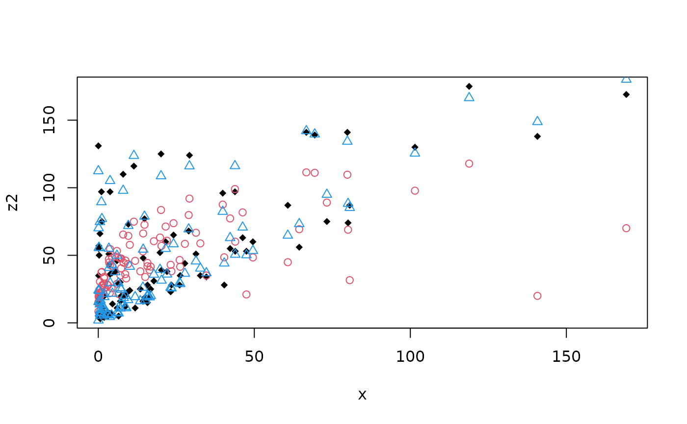
# Plotting the fits:
plot(x, z2, pch = 18)
points(x, fitted(est2_L), col = 2, pch = 1)
points(x, fitted(est2_NL), col = 4, pch = 2)