You can set the default values of most arguments of coefplot with this function.
setFixest_coefplot(
  style,
  horiz = FALSE,
  dict = getFixest_dict(),
  keep,
  ci.width = "1%",
  ci_level = 0.95,
  pt.pch = 20,
  pt.bg = NULL,
  cex = 1,
  pt.cex = cex,
  col = 1:8,
  pt.col = col,
  ci.col = col,
  lwd = 1,
  pt.lwd = lwd,
  ci.lwd = lwd,
  ci.lty = 1,
  grid = TRUE,
  grid.par = list(lty = 3, col = "gray"),
  zero = TRUE,
  zero.par = list(col = "black", lwd = 1),
  pt.join = FALSE,
  pt.join.par = list(col = pt.col, lwd = lwd),
  ci.join = FALSE,
  ci.join.par = list(lwd = lwd, col = col, lty = 2),
  ci.fill = FALSE,
  ci.fill.par = list(col = "lightgray", alpha = 0.5),
  ref.line = "auto",
  ref.line.par = list(col = "black", lty = 2),
  lab.cex,
  lab.min.cex = 0.85,
  lab.max.mar = 0.25,
  lab.fit = "auto",
  xlim.add,
  ylim.add,
  sep,
  bg,
  group = "auto",
  group.par = list(lwd = 2, line = 3, tcl = 0.75),
  main = "Effect on __depvar__",
  value.lab = "Estimate and __ci__ Conf. Int.",
  ylab = NULL,
  xlab = NULL,
  sub = NULL,
  reset = FALSE
)

getFixest_coefplot()
Arguments
- style
A character scalar giving the style of the plot to be used. You can set styles with the function
setFixest_coefplot, setting all the default values of the function. If missing, then it switches to either "default" or "iplot", depending on the calling function.- horiz
A logical scalar, default is
FALSE. Whether to display the confidence intervals horizontally instead of vertically.- dict
A named character vector or a logical scalar. It changes the original variable names to the ones contained in the
dictionary. E.g. to change the variables namedaandb3to (resp.) “$log(a)$” and to “$bonus^3$”, usedict=c(a="$log(a)$",b3="$bonus^3$"). By default, it is equal togetFixest_dict(), a default dictionary which can be set withsetFixest_dict. You can usedict = FALSEto disable it. By defaultdictmodifies the entries in the global dictionary, to disable this behavior, use "reset" as the first element (ex:dict=c("reset", mpg="Miles per gallon")).- keep
Character vector. This element is used to display only a subset of variables. This should be a vector of regular expressions (see
base::regexhelp for more info). Each variable satisfying any of the regular expressions will be kept. This argument is applied post aliasing (see argumentdict). Example: you have the variablex1tox55and want to display onlyx1tox9, then you could usekeep = "x[[:digit:]]$". If the first character is an exclamation mark, the effect is reversed (e.g. keep = "!Intercept" means: every variable that does not contain “Intercept” is kept). See details.- ci.width
The width of the extremities of the confidence intervals. Default is
0.1.- ci_level
Scalar between 0 and 1: the level of the CI. By default it is equal to 0.95.
- pt.pch
The patch of the coefficient estimates. Default is 1 (circle).
- pt.bg
The background color of the point estimate (when the
pt.pchis in 21 to 25). Defaults to NULL.- cex
Numeric, default is 1. Expansion factor for the points
- pt.cex
The size of the coefficient estimates. Default is the other argument
cex.- col
The color of the points and the confidence intervals. Default is 1 ("black"). Note that you can set the colors separately for each of them with
pt.colandci.col.- pt.col
The color of the coefficient estimates. Default is equal to the argument
col.- ci.col
The color of the confidence intervals. Default is equal to the argument
col.- lwd
General line with. Default is 1.
- pt.lwd
The line width of the coefficient estimates. Default is equal to the other argument
lwd.- ci.lwd
The line width of the confidence intervals. Default is equal to the other argument
lwd.- ci.lty
The line type of the confidence intervals. Default is 1.
- grid
Logical, default is
TRUE. Whether a grid should be displayed. You can set the display of the grid with the argumentgrid.par.- grid.par
List. Parameters of the grid. The default values are:
lty = 3andcol = "gray". You can add any graphical parameter that will be passed tographics::abline. You also have two additional arguments: usehoriz = FALSEto disable the horizontal lines, and usevert = FALSEto disable the vertical lines. Eg:grid.par = list(vert = FALSE, col = "red", lwd = 2).- zero
Logical, default is
TRUE. Whether the 0-line should be emphasized. You can set the parameters of that line with the argumentzero.par.- zero.par
List. Parameters of the zero-line. The default values are
col = "black"andlwd = 1. You can add any graphical parameter that will be passed tographics::abline. Example:zero.par = list(col = "darkblue", lwd = 3).- pt.join
Logical, default is
FALSE. IfTRUE, then the coefficient estimates are joined with a line.- pt.join.par
List. Parameters of the line joining the coefficients. The default values are:
col = pt.colandlwd = lwd. You can add any graphical parameter that will be passed tolines. Eg:pt.join.par = list(lty = 2).- ci.join
Logical default to
FALSE. Whether to join the extremities of the confidence intervals. IfTRUE, then you can set the graphical parameters with the argumentci.join.par.- ci.join.par
A list of parameters to be passed to
graphics::lines. Only used ifci.join=TRUE. By default it is equal tolist(lwd = lwd, col = col, lty = 2).- ci.fill
Logical default to
FALSE. Whether to fill the confidence intervals with a color. IfTRUE, then you can set the graphical parameters with the argumentci.fill.par.- ci.fill.par
A list of parameters to be passed to
graphics::polygon. Only used ifci.fill=TRUE. By default it is equal tolist(col = "lightgray", alpha = 0.5). Note thatalphais a special parameter that adds transparency to the color (ranges from 0 to 1).- ref.line
Logical or numeric, default is "auto", whose behavior depends on the situation. It is
TRUEonly if: i) interactions are plotted, ii) the x values are numeric and iii) a reference is found. IfTRUE, then a vertical line is drawn at the level of the reference value. Otherwise, if numeric a vertical line will be drawn at that specific value.- ref.line.par
List. Parameters of the vertical line on the reference. The default values are:
col = "black"andlty = 2. You can add any graphical parameter that will be passed tographics::abline. Eg:ref.line.par = list(lty = 1, lwd = 3).- lab.cex
The size of the labels of the coefficients. Default is missing. It is automatically set by an internal algorithm which can go as low as
lab.min.cex(another argument).- lab.min.cex
The minimum size of the coefficients labels, as set by the internal algorithm. Default is 0.85.
- lab.max.mar
The maximum size the left margin can take when trying to fit the coefficient labels into it (only when
horiz = TRUE). This is used in the internal algorithm fitting the coefficient labels. Default is0.25.- lab.fit
The method to fit the coefficient labels into the plotting region (only when
horiz = FALSE). Can be"auto"(the default),"simple","multi"or"tilted". If"simple", then the classic axis is drawn. If"multi", then the coefficient labels are fit horizontally across several lines, such that they don't collide. If"tilted", then the labels are tilted. If"auto", an automatic choice between the three is made.- xlim.add
A numeric vector of length 1 or 2. It represents an extension factor of xlim, in percentage. Eg:
xlim.add = c(0, 0.5)extendsxlimof 50% on the right. If of length 1, positive values represent the right, and negative values the left (Eg:xlim.add = -0.5is equivalent toxlim.add = c(0.5, 0)).- ylim.add
A numeric vector of length 1 or 2. It represents an extension factor of ylim, in percentage. Eg:
ylim.add = c(0, 0.5)extendsylimof 50% on the top. If of length 1, positive values represent the top, and negative values the bottom (Eg:ylim.add = -0.5is equivalent toylim.add = c(0.5, 0)).- sep
The distance between two estimates – only when argument
objectis a list of estimation results.- bg
Background color for the plot. By default it is white.
- group
A list, default is missing. Each element of the list reports the coefficients to be grouped while the name of the element is the group name. Each element of the list can be either: i) a character vector of length 1, ii) of length 2, or ii) a numeric vector. If equal to: i) then it is interpreted as a pattern: all element fitting the regular expression will be grouped (note that you can use the special character "^^" to clean the beginning of the names, see example), if ii) it corresponds to the first and last elements to be grouped, if iii) it corresponds to the coefficients numbers to be grouped. If equal to a character vector, you can use a percentage to tell the algorithm to look at the coefficients before aliasing (e.g.
"%varname"). Example of valid uses:group=list(group_name=\"pattern\"),group=list(group_name=c(\"var_start\", \"var_end\")),group=list(group_name=1:2)). See details.- group.par
A list of parameters controlling the display of the group. The parameters controlling the line are:
lwd,tcl(length of the tick),line.adj(adjustment of the position, default is 0),tick(whether to add the ticks),lwd.ticks,col.ticks. Then the parameters controlling the text:text.adj(adjustment of the position, default is 0),text.cex,text.font,text.col.- main
The title of the plot. Default is
"Effect on __depvar__". You can use the special variable__depvar__to set the title (useful when you set the plot default withsetFixest_coefplot).- value.lab
The label to appear on the side of the coefficient values. If
horiz = FALSE, the label appears in the y-axis. Ifhoriz = TRUE, then it appears on the x-axis. The default is equal to"Estimate and __ci__ Conf. Int.", with__ci__a special variable giving the value of the confidence interval.- ylab
The label of the y-axis, default is
NULL. Note that ifhoriz = FALSE, it overrides the value of the argumentvalue.lab.- xlab
The label of the x-axis, default is
NULL. Note that ifhoriz = TRUE, it overrides the value of the argumentvalue.lab.- sub
A subtitle, default is
NULL.- reset
Logical, default is
TRUE. IfTRUE, then the arguments that are not set during the call are reset to their "factory"-default values. IfFALSE, on the other hand, arguments that have already been modified are not changed.
Value
Doesn't return anything.
See also
Examples
# coefplot has many arguments, which makes it highly flexible.
# If you don't like the default style of coefplot. No worries,
# you can set *your* default by using the function
# setFixest_coefplot()
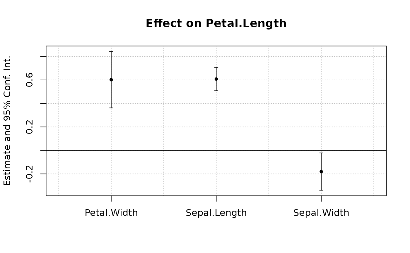
# Estimation
est = feols(Petal.Length ~ Petal.Width + Sepal.Length +
Sepal.Width | Species, iris)
# Plot with default style
coefplot(est)
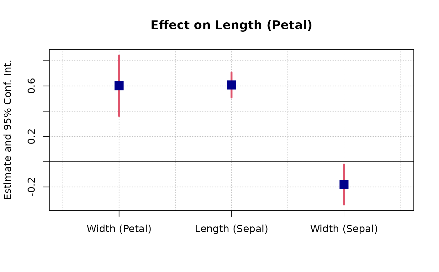
 # Now we permanently change some arguments
dict = c("Petal.Length"="Length (Petal)", "Petal.Width"="Width (Petal)",
"Sepal.Length"="Length (Sepal)", "Sepal.Width"="Width (Sepal)")
setFixest_coefplot(ci.col = 2, pt.col = "darkblue", ci.lwd = 3,
pt.cex = 2, pt.pch = 15, ci.width = 0, dict = dict)
# Tadaaa!
coefplot(est)
# Now we permanently change some arguments
dict = c("Petal.Length"="Length (Petal)", "Petal.Width"="Width (Petal)",
"Sepal.Length"="Length (Sepal)", "Sepal.Width"="Width (Sepal)")
setFixest_coefplot(ci.col = 2, pt.col = "darkblue", ci.lwd = 3,
pt.cex = 2, pt.pch = 15, ci.width = 0, dict = dict)
# Tadaaa!
coefplot(est)
 # To reset to the default settings:
setFixest_coefplot("all", reset = TRUE)
coefplot(est)
# To reset to the default settings:
setFixest_coefplot("all", reset = TRUE)
coefplot(est)
