FlexMix Clustering Demo Driver

These are demo drivers for flexmix implementing model-based clustering of Gaussian data.

FLXMCmvnorm(formula = . ~ ., diagonal = TRUE)
FLXMCnorm1(formula = . ~ .)

Arguments

formula: A formula which is interpreted relative to the formula specified in the call to flexmix using update.formula. Only the left-hand side (response) of the formula is used. Default is to use the original flexmix model formula.
diagonal: If TRUE, then the covariance matrix of the components is restricted to diagonal matrices.

Details

This is mostly meant as a demo for FlexMix driver programming, you should also look at package mclust for real applications. FLXMCmvnorm clusters multivariate data, FLXMCnorm1 univariate data. In the latter case smart initialization is important, see the example below.

Value

FLXMCmvnorm returns an object of class FLXMC.

Author

Friedrich Leisch and Bettina Gruen

References

Friedrich Leisch. FlexMix: A general framework for finite mixture models and latent class regression in R. Journal of Statistical Software, 11(8), 2004. doi:10.18637/jss.v011.i08

Examples

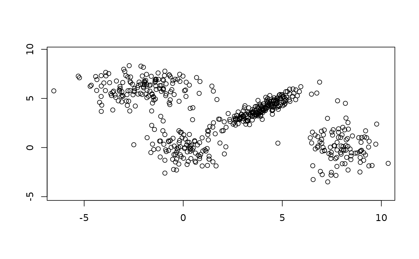
data("Nclus", package = "flexmix")

require("MASS")
eqscplot(Nclus)


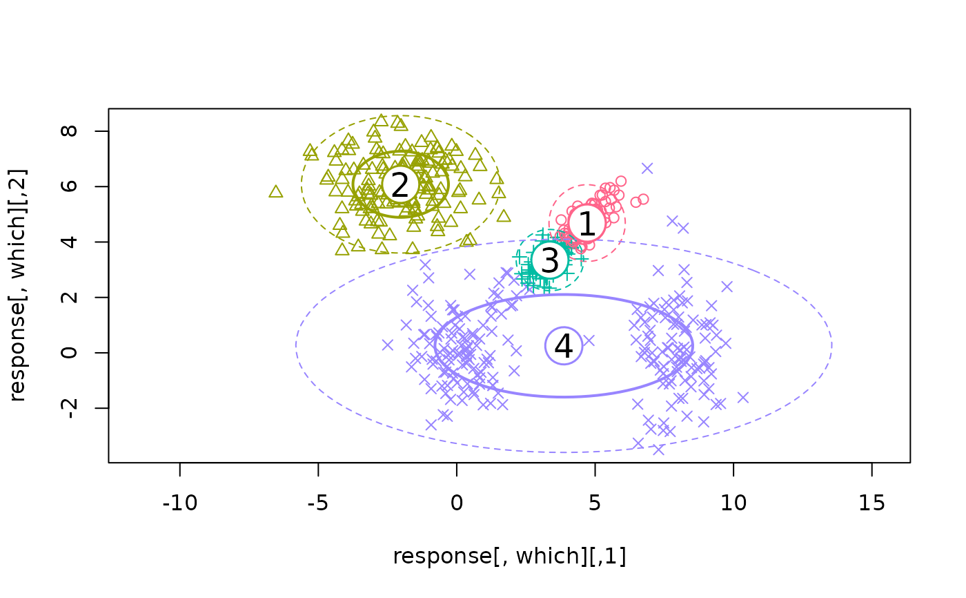
## This model is wrong (one component has a non-diagonal cov matrix)
ex1 <- flexmix(Nclus ~ 1, k = 4, model = FLXMCmvnorm())
print(ex1)
#> 
#> Call:
#> flexmix(formula = Nclus ~ 1, k = 4, model = FLXMCmvnorm())
#> 
#> Cluster sizes:
#>   1   2   3   4 
#>  96 149  92 213 
#> 
#> convergence after 194 iterations
plotEll(ex1, Nclus)


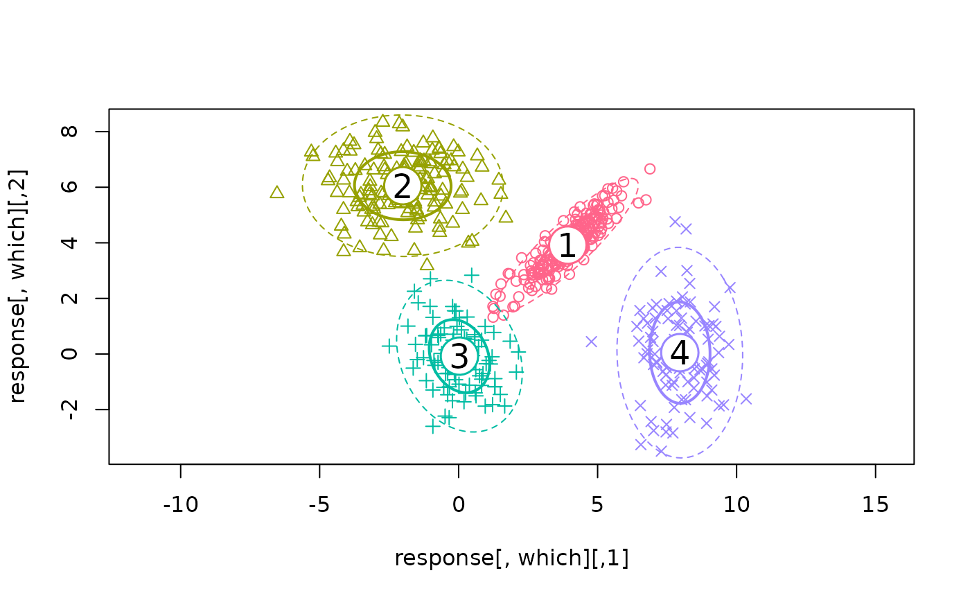
## True model, wrong number of components
ex2 <- flexmix(Nclus ~ 1, k = 6, model = FLXMCmvnorm(diagonal = FALSE))  
print(ex2)
#> 
#> Call:
#> flexmix(formula = Nclus ~ 1, k = 6, model = FLXMCmvnorm(diagonal = FALSE))
#> 
#> Cluster sizes:
#>   1   2   3   4 
#> 204 150  96 100 
#> 
#> convergence after 26 iterations

plotEll(ex2, Nclus)


## Get parameters of first component
parameters(ex2, component = 1)
#>            Comp.1
#> center1 3.9270274
#> center2 3.9177159
#> cov1    1.0737947
#> cov2    0.9109258
#> cov3    0.9109258
#> cov4    0.9604122

## Have a look at the posterior probabilies of 10 random observations
ok <- sample(1:nrow(Nclus), 10)
p  <- posterior(ex2)[ok, ]
p
#>                [,1]         [,2]         [,3]         [,4]
#>  [1,] 2.666664e-135 5.358805e-26 6.475614e-20 1.000000e+00
#>  [2,]  3.459977e-07 2.271399e-11 9.999997e-01 1.900477e-15
#>  [3,]  1.359455e-55 1.000000e+00 4.095438e-09 3.450189e-22
#>  [4,]  1.714111e-88 3.551478e-20 1.179123e-21 1.000000e+00
#>  [5,] 5.734686e-128 1.000000e+00 2.358708e-11 3.675333e-40
#>  [6,]  5.154188e-08 1.768465e-12 9.999999e-01 9.534319e-18
#>  [7,]  9.999906e-01 8.832400e-06 1.310348e-09 5.723562e-07
#>  [8,]  9.999382e-01 6.020852e-05 6.204183e-12 1.635255e-06
#>  [9,] 4.789248e-102 6.547787e-22 8.501703e-21 1.000000e+00
#> [10,]  9.999926e-01 6.017151e-06 2.752451e-09 1.418790e-06

## The following two should be the same
max.col(p)
#>  [1] 4 3 2 4 2 3 1 1 4 1
clusters(ex2)[ok]
#>  [1] 4 3 2 4 2 3 1 1 4 1
## Now try the univariate case
plot(density(Nclus[, 1]))


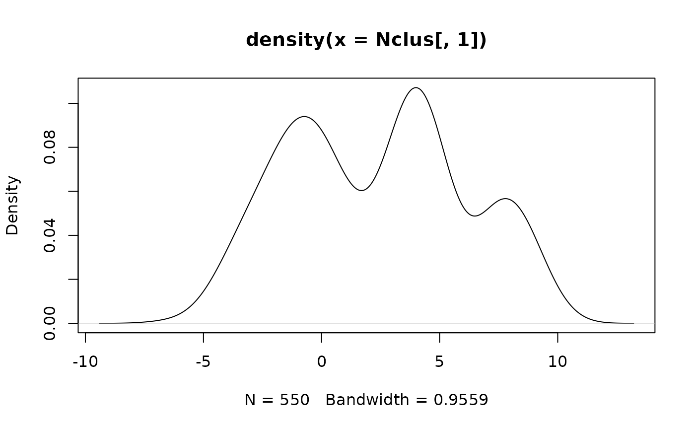ex3 <- flexmix(Nclus[, 1] ~ 1, cluster = cut(Nclus[, 1], 3),
               model = FLXMCnorm1())
ex3
#> 
#> Call:
#> flexmix(formula = Nclus[, 1] ~ 1, cluster = cut(Nclus[, 1], 3), 
#>     model = FLXMCnorm1())
#> 
#> Cluster sizes:
#>   1   2   3 
#> 262 186 102 
#> 
#> convergence after 128 iterations
parameters(ex3)
#>          Comp.1    Comp.2    Comp.3
#> mean -0.9217948 4.0600622 7.9189585
#> sd    1.8563637 0.8391779 0.9286542