Random Number Generator for Finite Mixtures

Given a finite mixture model generate random numbers from it.

rflexmix(object, newdata, ...)

Arguments

object

A fitted finite mixture model of class flexmix or an unfitted of class FLXdist.

newdata

Optionally, a data frame in which to look for variables with which to predict or an integer specifying the number of random draws for model-based clustering. If omitted, the data to which the model was fitted is used.

...

Further arguments to be passed to or from methods.

Details

rflexmix provides the creation of the model matrix for new data and the sampling of the cluster memberships. The sampling of the component distributions given the classification is done by calling rFLXM. This step has to be provided for the different model classes.

Value

A list with components

y

Random sample

group

Grouping factor

class

Class membership

Author

Bettina Gruen

Examples

example(flexmix)
#> 
#> flexmx> data("NPreg", package = "flexmix")
#> 
#> flexmx> ## mixture of two linear regression models. Note that control parameters
#> flexmx> ## can be specified as named list and abbreviated if unique.
#> flexmx> ex1 <- flexmix(yn ~ x + I(x^2), data = NPreg, k = 2,
#> flexmx+                control = list(verb = 5, iter = 100))
#> Classification: weighted 
#>    5 Log-likelihood :    -722.2404 
#>   10 Log-likelihood :    -656.0035 
#>   15 Log-likelihood :    -642.5457 
#>   16 Log-likelihood :    -642.5453 
#> converged
#> 
#> flexmx> ex1
#> 
#> Call:
#> flexmix(formula = yn ~ x + I(x^2), data = NPreg, k = 2, control = list(verb = 5, 
#>     iter = 100))
#> 
#> Cluster sizes:
#>   1   2 
#> 100 100 
#> 
#> convergence after 16 iterations
#> 
#> flexmx> summary(ex1)
#> 
#> Call:
#> flexmix(formula = yn ~ x + I(x^2), data = NPreg, k = 2, control = list(verb = 5, 
#>     iter = 100))
#> 
#>        prior size post>0 ratio
#> Comp.1 0.494  100    145 0.690
#> Comp.2 0.506  100    141 0.709
#> 
#> 'log Lik.' -642.5453 (df=9)
#> AIC: 1303.091   BIC: 1332.776 
#> 
#> 
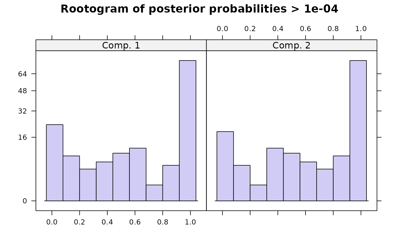
#> flexmx> plot(ex1)

#> 
#> flexmx> ## now we fit a model with one Gaussian response and one Poisson
#> flexmx> ## response. Note that the formulas inside the call to FLXMRglm are
#> flexmx> ## relative to the overall model formula.
#> flexmx> ex2 <- flexmix(yn ~ x, data = NPreg, k = 2,
#> flexmx+                model = list(FLXMRglm(yn ~ . + I(x^2)), 
#> flexmx+                             FLXMRglm(yp ~ ., family = "poisson")))
#> 
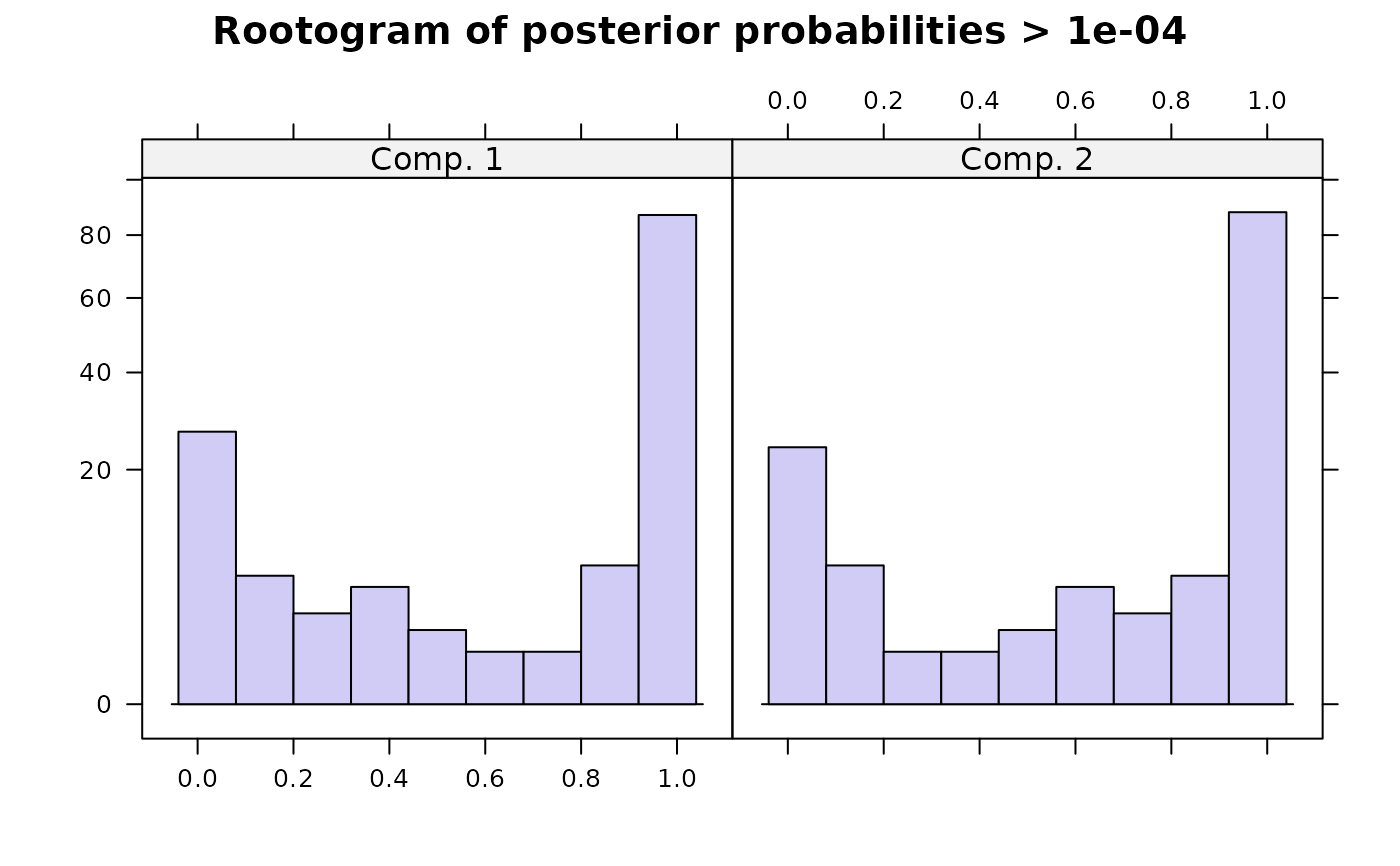
#> flexmx> plot(ex2)

#> 
#> flexmx> ex2
#> 
#> Call:
#> flexmix(formula = yn ~ x, data = NPreg, k = 2, model = list(FLXMRglm(yn ~ 
#>     . + I(x^2)), FLXMRglm(yp ~ ., family = "poisson")))
#> 
#> Cluster sizes:
#>   1   2 
#>  96 104 
#> 
#> convergence after 11 iterations
#> 
#> flexmx> table(ex2@cluster, NPreg$class)
#>    
#>      1  2
#>   1  1 95
#>   2 99  5
#> 
#> flexmx> ## for Gaussian responses we get coefficients and standard deviation
#> flexmx> parameters(ex2, component = 1, model = 1)
#>                      Comp.1
#> coef.(Intercept) 14.5914766
#> coef.x            9.9146975
#> coef.I(x^2)      -0.9756903
#> sigma             3.4115522
#> 
#> flexmx> ## for Poisson response we get only coefficients
#> flexmx> parameters(ex2, component = 1, model = 2)
#>                      Comp.1
#> coef.(Intercept) 1.03770716
#> coef.x           0.09106366
#> 
#> flexmx> ## fitting a model only to the Poisson response is of course
#> flexmx> ## done like this
#> flexmx> ex3 <- flexmix(yp ~ x, data = NPreg, k = 2,
#> flexmx+                model = FLXMRglm(family = "poisson"))
#> 
#> flexmx> ## if observations are grouped, i.e., we have several observations per
#> flexmx> ## individual, fitting is usually much faster:
#> flexmx> ex4 <- flexmix(yp~x|id1, data = NPreg, k = 2,
#> flexmx+                model = FLXMRglm(family = "poisson"))
#> 
#> flexmx> ## And now a binomial example. Mixtures of binomials are not generically
#> flexmx> ## identified, here the grouping variable is necessary:
#> flexmx> set.seed(1234)
#> 
#> flexmx> ex5 <- initFlexmix(cbind(yb,1 - yb) ~ x, data = NPreg, k = 2,
#> flexmx+                    model = FLXMRglm(family = "binomial"), nrep = 5)
#> 2 : * * * * *
#> 
#> flexmx> table(NPreg$class, clusters(ex5))
#>    
#>       1   2
#>   1   0 100
#>   2   9  91
#> 
#> flexmx> ex6 <- initFlexmix(cbind(yb, 1 - yb) ~ x | id2, data = NPreg, k = 2,
#> flexmx+                    model = FLXMRglm(family = "binomial"), nrep = 5)
#> 2 : * * * * *
#> 
#> flexmx> table(NPreg$class, clusters(ex6))
#>    
#>      1  2
#>   1 92  8
#>   2  4 96
sample <- rflexmix(ex1)