Epileptic Seizure Data

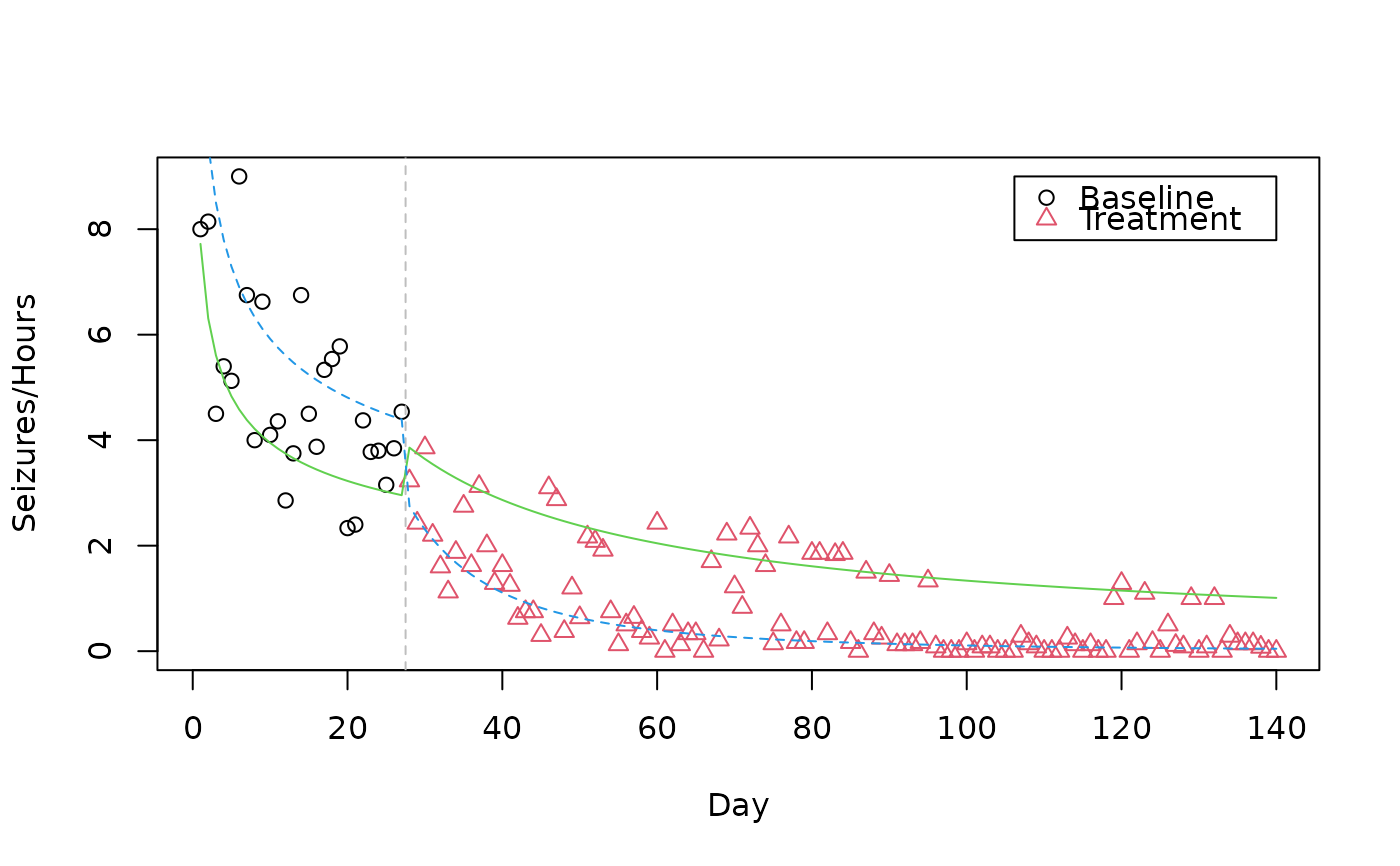
Data from a clinical trial where the effect of intravenous gamma-globulin on suppression of epileptic seizures is studied. Daily observations for a period of 140 days on one patient are given, where the first 27 days are a baseline period without treatment, the remaining 113 days are the treatment period.

data("seizure")

Format

A data frame with 140 observations on the following 4 variables.

Seizures

A numeric vector, daily counts of epileptic seizures.

Hours

A numeric vector, hours of daily parental observation.

Treatment

A factor with levels No and Yes.

Day

A numeric vector.

Source

P. Wang, M. Puterman, I. Cockburn, and N. Le. Mixed poisson regression models with covariate dependent rates. Biometrics, 52, 381–400, 1996.

References

B. Gruen and F. Leisch. Bootstrapping finite mixture models. In J. Antoch, editor, Compstat 2004–Proceedings in Computational Statistics, 1115–1122. Physika Verlag, Heidelberg, Germany, 2004. ISBN 3-7908-1554-3.

Examples

data("seizure", package = "flexmix")
plot(Seizures/Hours ~ Day, col = as.integer(Treatment),
     pch = as.integer(Treatment), data = seizure)
abline(v = 27.5, lty = 2, col = "grey")
legend(140, 9, c("Baseline", "Treatment"),
       pch = 1:2, col = 1:2, xjust = 1, yjust = 1)

set.seed(123)

## The model presented in the Wang et al paper: two components for
## "good" and "bad" days, respectively, each a Poisson GLM with hours of
## parental observation as offset

seizMix <- flexmix(Seizures ~ Treatment * log(Day),
                   data = seizure, k = 2,
                   model = FLXMRglm(family = "poisson",
                     offset = log(seizure$Hours)))

summary(seizMix)
#> 
#> Call:
#> flexmix(formula = Seizures ~ Treatment * log(Day), data = seizure, 
#>     k = 2, model = FLXMRglm(family = "poisson", offset = log(seizure$Hours)))
#> 
#>        prior size post>0 ratio
#> Comp.1 0.307   42    108 0.389
#> Comp.2 0.693   98    116 0.845
#> 
#> 'log Lik.' -380.7697 (df=9)
#> AIC: 779.5393   BIC: 806.0141 
#> 
summary(refit(seizMix))
#> $Comp.1
#>                        Estimate Std. Error z value  Pr(>|z|)    
#> (Intercept)            2.043989   0.120852 16.9132 < 2.2e-16 ***
#> TreatmentYes           2.081361   0.495066  4.2042 2.620e-05 ***
#> log(Day)              -0.291203   0.057822 -5.0362 4.749e-07 ***
#> TreatmentYes:log(Day) -0.541596   0.128682 -4.2088 2.567e-05 ***
#> ---
#> Signif. codes:  0 ‘***’ 0.001 ‘**’ 0.01 ‘*’ 0.05 ‘.’ 0.1 ‘ ’ 1
#> 
#> $Comp.2
#>                        Estimate Std. Error  z value  Pr(>|z|)    
#> (Intercept)            2.470428   0.242776  10.1757 < 2.2e-16 ***
#> TreatmentYes           7.025729   0.597897  11.7507 < 2.2e-16 ***
#> log(Day)              -0.300391   0.086015  -3.4923 0.0004789 ***
#> TreatmentYes:log(Day) -2.245671   0.166680 -13.4729 < 2.2e-16 ***
#> ---
#> Signif. codes:  0 ‘***’ 0.001 ‘**’ 0.01 ‘*’ 0.05 ‘.’ 0.1 ‘ ’ 1
#> 

matplot(seizure$Day, fitted(seizMix)/seizure$Hours, type = "l",
        add = TRUE, col = 3:4)