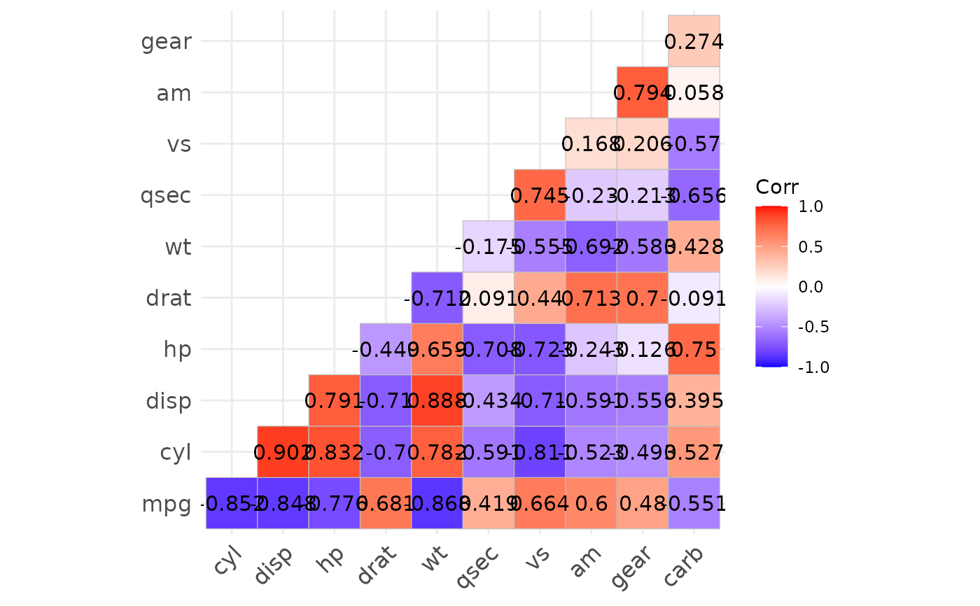
ggcorrplot(): A graphical display of a correlation matrix using ggplot2.
cor_pmat(): Compute a correlation matrix p-values.
Usage
ggcorrplot(
  corr,
  method = c("square", "circle"),
  type = c("full", "lower", "upper"),
  ggtheme = ggplot2::theme_minimal,
  title = "",
  show.legend = TRUE,
  legend.title = "Corr",
  show.diag = NULL,
  colors = c("blue", "white", "red"),
  outline.color = "gray",
  hc.order = FALSE,
  hc.method = "complete",
  lab = FALSE,
  lab_col = "black",
  lab_size = 4,
  lab_fontface = "plain",
  sig.stars = FALSE,
  p.mat = NULL,
  sig.level = 0.05,
  insig = c("pch", "blank"),
  pch = 4,
  pch.col = "black",
  pch.cex = 5,
  tl.cex = 12,
  tl.col = NULL,
  tl.srt = 45,
  tl.vjust = 1,
  tl.hjust = 1,
  digits = 2,
  as.is = FALSE,
  nsmall = 0L,
  leading.zero = TRUE,
  legend.limit = c(-1, 1),
  circle.scale = 1,
  coord.fixed = TRUE
)

cor_pmat(x, ..., use = c("pairwise.complete.obs", "everything"))
Arguments
- corr
the correlation matrix to visualize
- method
character, the visualization method of correlation matrix to be used. Allowed values are "square" (default), "circle".
- type
character, "full" (default), "lower" or "upper" display.
- ggtheme
ggplot2 function or theme object. Default value is `theme_minimal`. Allowed values are the official ggplot2 themes including theme_gray, theme_bw, theme_minimal, theme_classic, theme_void, .... Theme objects are also allowed (e.g., `theme_classic()`).
- title
character, title of the graph.
- show.legend
logical, if TRUE the legend is displayed.
- legend.title
a character string for the legend title. lower triangular, upper triangular or full matrix.
- show.diag
NULL or logical, whether display the correlation coefficients on the principal diagonal. If
NULL, the default is to show diagonal correlation fortype = "full"and to remove it whentypeis one of "upper" or "lower".- colors
a vector of colors for the fill gradient. The default is a length-3 vector for the low, mid and high correlation values (mapped with
scale_fill_gradient2). A vector of any other length (>= 2) is spread evenly across the scale withscale_fill_gradientn, so an n-color palette (e.g.RColorBrewer::brewer.pal(11, "RdBu")) can be passed directly.- outline.color
the outline color of square or circle. Default value is "gray".
- hc.order
logical value. If TRUE, correlation matrix will be hc.ordered using hclust function.
- hc.method
the agglomeration method to be used in hclust (see ?hclust).
- lab
logical value. If TRUE, add correlation coefficient on the plot.
- lab_col, lab_size
size and color to be used for the correlation coefficient labels. used when lab = TRUE.
- lab_fontface
the font face (
"plain","bold","italic","bold.italic") for the correlation coefficient labels. Default is"plain". Used whenlab = TRUE.- sig.stars
logical value. If
TRUEand ap.matis supplied, significance stars are appended to the coefficient labels (***for p < 0.001,**for p < 0.01,*for p < 0.05), e.g."-0.85**". Only used whenlab = TRUE. Default isFALSE. WhenTRUE, significance is shown by the stars and theinsig = "pch"markers are not drawn.- p.mat
matrix of p-value. If NULL, arguments sig.level, insig, pch, pch.col, pch.cex is invalid.
- sig.level
significant level, if the p-value in p-mat is bigger than sig.level, then the corresponding correlation coefficient is regarded as insignificant.
- insig
character, specialized insignificant correlation coefficients, "pch" (default), "blank". If "blank", wipe away the corresponding glyphs; if "pch", add characters (see pch for details) on corresponding glyphs.
- pch
add character on the glyphs of insignificant correlation coefficients (only valid when insig is "pch"). Default value is 4.
- pch.col, pch.cex
the color and the cex (size) of pch (only valid when insig is "pch").
- tl.cex, tl.col, tl.srt
the size, the color and the string rotation of text label (variable names).
tl.coldefaults toNULL, which inherits the color from the theme.- tl.vjust, tl.hjust
the vertical and horizontal justification of the x-axis text labels, passed to
element_text. Both default to1; adjust them to reposition the variable-name labels.- digits
Decides the number of decimal digits to be displayed (Default: `2`).
- as.is
A logical passed to
melt.array. IfTRUE, dimnames will be left as strings instead of being converted usingtype.convert.- nsmall
the minimum number of digits to the right of the decimal point in the coefficient labels, passed to
format. Default is0(no minimum, current behavior). Set e.g.nsmall = 2to keep trailing zeros (such as 0.70). Only used whenlab = TRUE.- leading.zero
logical. If
TRUE(default), coefficient labels keep the leading zero (e.g.0.23,-0.67). Set toFALSEto drop it (.23,-.67), which is common for correlation tables. Only used whenlab = TRUE.- legend.limit
a length-2 numeric vector giving the limits of the fill color scale. Default
c(-1, 1)(suitable for a correlation matrix); set toNULLto use the data range instead, e.g. for a covariance matrix.- circle.scale
a scaling factor for the circle sizes when
method = "circle". Default is1; increase it (e.g.circle.scale = 2) for larger circles or decrease it for smaller ones, which is useful when the output device size makes the default circles too small or too large. Has no effect whenmethod = "square".- coord.fixed
logical value. If
TRUE(default), the plot usescoord_fixedso the cells are square. Set toFALSEto let the cells fill the plotting area (a non 1:1 aspect ratio), which can look better with many long variable names.- x
numeric matrix or data frame
- ...
other arguments to be passed to the function cor.test.
- use
character, how to treat pairs involving missing values when deciding which cells are
NA. Either"pairwise.complete.obs"(default; test every pair that has enough overlapping observations) or"everything"(set a pair toNAas soon as either variable has a missing value, matchingcor's default). Mirrors the corresponding values ofcor'suseargument.
Value
ggcorrplot(): Returns a ggplot2
cor_pmat(): Returns a matrix containing the p-values of correlations
Details
cor_pmat() tests each pair of columns with
cor.test. A pair with fewer than three overlapping
non-missing observations (which cor.test cannot test,
e.g. two variables that never co-occur) yields NA for that cell
rather than aborting the whole computation. Pairs that can be tested are
computed as before, and errors they raise are passed through.
The use argument controls which pairs are returned as NA so
the p-value matrix can be aligned with a correlation matrix built the same
way. With the default "pairwise.complete.obs" every pair that has
enough overlapping observations is tested (the previous behavior). With
"everything" a pair is set to NA whenever either variable has
any missing value, so the NA pattern matches
cor(x) with its default use = "everything".
Examples
# Compute a correlation matrix
data(mtcars)
corr <- round(cor(mtcars), 1)
corr
#> mpg cyl disp hp drat wt qsec vs am gear carb
#> mpg 1.0 -0.9 -0.8 -0.8 0.7 -0.9 0.4 0.7 0.6 0.5 -0.6
#> cyl -0.9 1.0 0.9 0.8 -0.7 0.8 -0.6 -0.8 -0.5 -0.5 0.5
#> disp -0.8 0.9 1.0 0.8 -0.7 0.9 -0.4 -0.7 -0.6 -0.6 0.4
#> hp -0.8 0.8 0.8 1.0 -0.4 0.7 -0.7 -0.7 -0.2 -0.1 0.7
#> drat 0.7 -0.7 -0.7 -0.4 1.0 -0.7 0.1 0.4 0.7 0.7 -0.1
#> wt -0.9 0.8 0.9 0.7 -0.7 1.0 -0.2 -0.6 -0.7 -0.6 0.4
#> qsec 0.4 -0.6 -0.4 -0.7 0.1 -0.2 1.0 0.7 -0.2 -0.2 -0.7
#> vs 0.7 -0.8 -0.7 -0.7 0.4 -0.6 0.7 1.0 0.2 0.2 -0.6
#> am 0.6 -0.5 -0.6 -0.2 0.7 -0.7 -0.2 0.2 1.0 0.8 0.1
#> gear 0.5 -0.5 -0.6 -0.1 0.7 -0.6 -0.2 0.2 0.8 1.0 0.3
#> carb -0.6 0.5 0.4 0.7 -0.1 0.4 -0.7 -0.6 0.1 0.3 1.0
# Compute a matrix of correlation p-values
p.mat <- cor_pmat(mtcars)
p.mat
#> mpg cyl disp hp drat
#> mpg 0.000000e+00 6.112687e-10 9.380327e-10 1.787835e-07 1.776240e-05
#> cyl 6.112687e-10 0.000000e+00 1.802838e-12 3.477861e-09 8.244636e-06
#> disp 9.380327e-10 1.802838e-12 0.000000e+00 7.142679e-08 5.282022e-06
#> hp 1.787835e-07 3.477861e-09 7.142679e-08 0.000000e+00 9.988772e-03
#> drat 1.776240e-05 8.244636e-06 5.282022e-06 9.988772e-03 0.000000e+00
#> wt 1.293959e-10 1.217567e-07 1.222320e-11 4.145827e-05 4.784260e-06
#> qsec 1.708199e-02 3.660533e-04 1.314404e-02 5.766253e-06 6.195826e-01
#> vs 3.415937e-05 1.843018e-08 5.235012e-06 2.940896e-06 1.167553e-02
#> am 2.850207e-04 2.151207e-03 3.662114e-04 1.798309e-01 4.726790e-06
#> gear 5.400948e-03 4.173297e-03 9.635921e-04 4.930119e-01 8.360110e-06
#> carb 1.084446e-03 1.942340e-03 2.526789e-02 7.827810e-07 6.211834e-01
#> wt qsec vs am gear
#> mpg 1.293959e-10 1.708199e-02 3.415937e-05 2.850207e-04 5.400948e-03
#> cyl 1.217567e-07 3.660533e-04 1.843018e-08 2.151207e-03 4.173297e-03
#> disp 1.222320e-11 1.314404e-02 5.235012e-06 3.662114e-04 9.635921e-04
#> hp 4.145827e-05 5.766253e-06 2.940896e-06 1.798309e-01 4.930119e-01
#> drat 4.784260e-06 6.195826e-01 1.167553e-02 4.726790e-06 8.360110e-06
#> wt 0.000000e+00 3.388683e-01 9.798492e-04 1.125440e-05 4.586601e-04
#> qsec 3.388683e-01 0.000000e+00 1.029669e-06 2.056621e-01 2.425344e-01
#> vs 9.798492e-04 1.029669e-06 0.000000e+00 3.570439e-01 2.579439e-01
#> am 1.125440e-05 2.056621e-01 3.570439e-01 0.000000e+00 5.834043e-08
#> gear 4.586601e-04 2.425344e-01 2.579439e-01 5.834043e-08 0.000000e+00
#> carb 1.463861e-02 4.536949e-05 6.670496e-04 7.544526e-01 1.290291e-01
#> carb
#> mpg 1.084446e-03
#> cyl 1.942340e-03
#> disp 2.526789e-02
#> hp 7.827810e-07
#> drat 6.211834e-01
#> wt 1.463861e-02
#> qsec 4.536949e-05
#> vs 6.670496e-04
#> am 7.544526e-01
#> gear 1.290291e-01
#> carb 0.000000e+00
# Visualize the correlation matrix
# --------------------------------
# method = "square" or "circle"
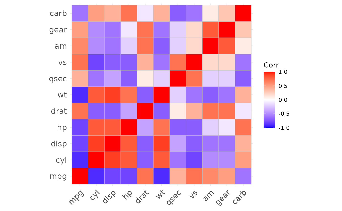
ggcorrplot(corr)
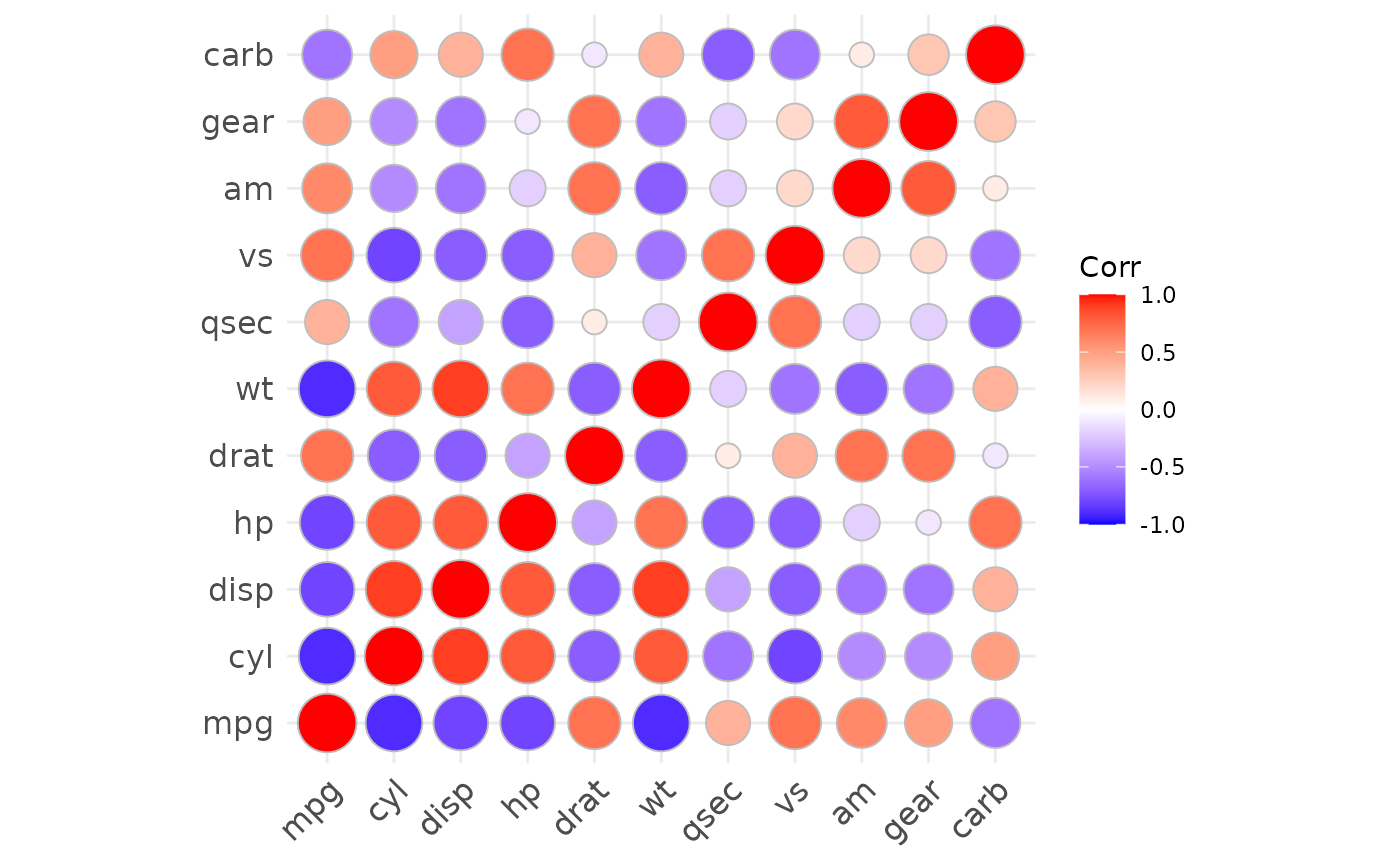
 ggcorrplot(corr, method = "circle")
 # Reordering the correlation matrix
# --------------------------------
# using hierarchical clustering
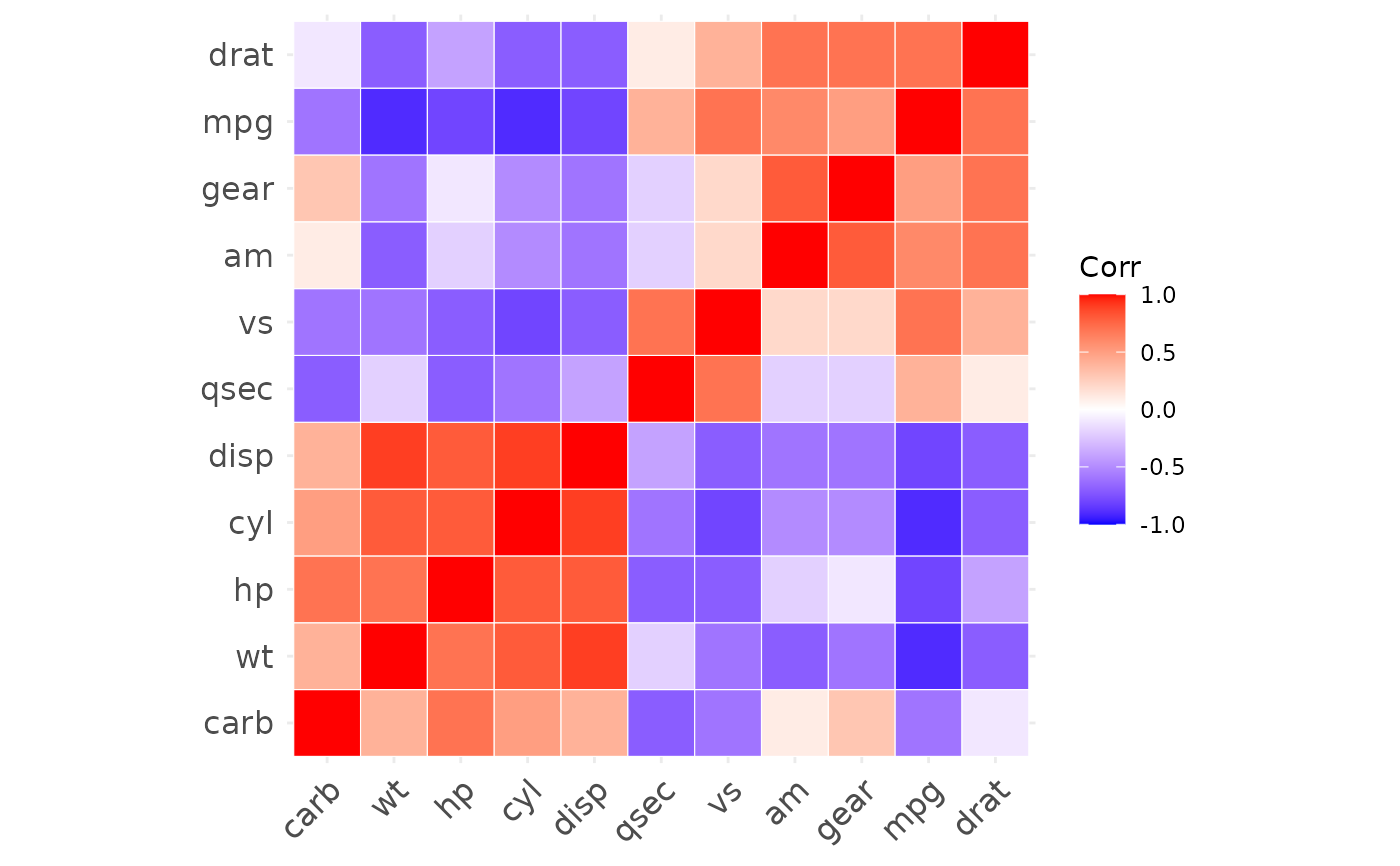
ggcorrplot(corr, hc.order = TRUE, outline.color = "white")
# Reordering the correlation matrix
# --------------------------------
# using hierarchical clustering
ggcorrplot(corr, hc.order = TRUE, outline.color = "white")
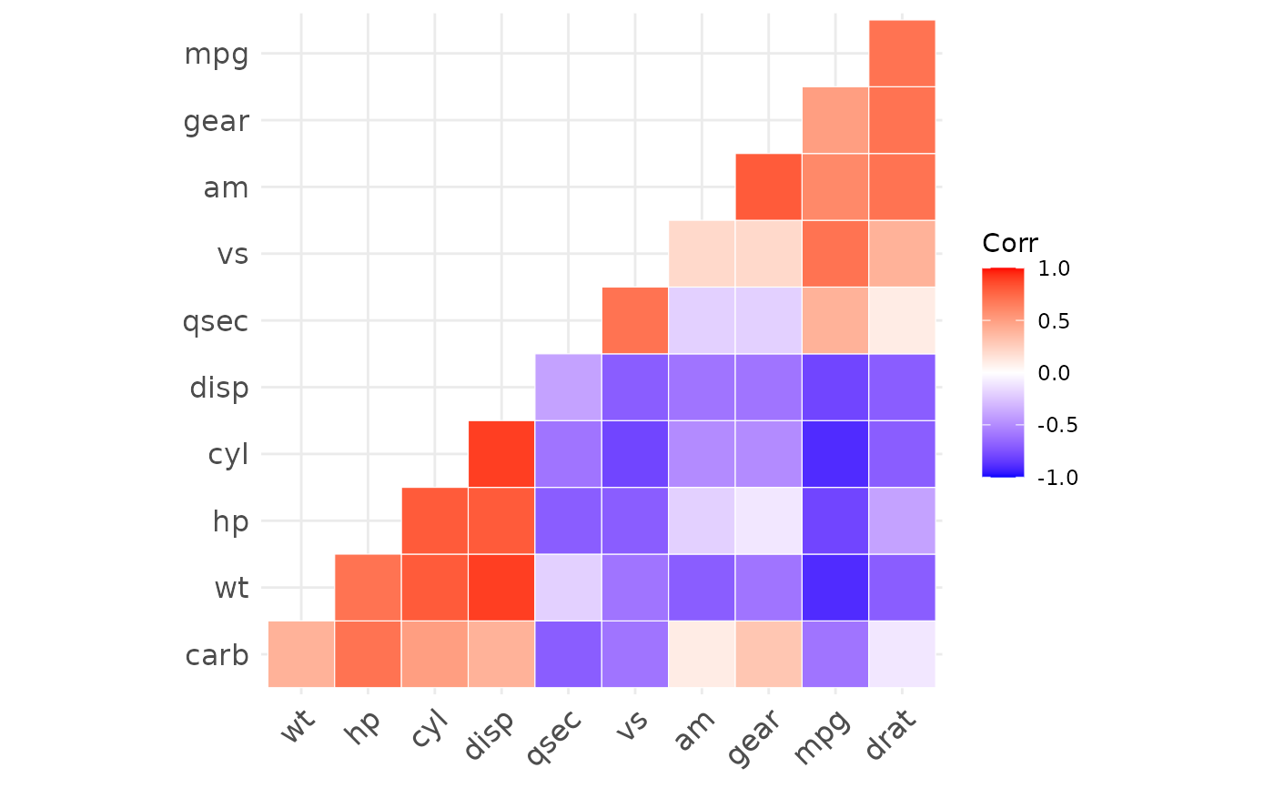
 # Types of correlogram layout
# --------------------------------
# Get the lower triangle
ggcorrplot(corr,
hc.order = TRUE, type = "lower",
outline.color = "white"
)
# Types of correlogram layout
# --------------------------------
# Get the lower triangle
ggcorrplot(corr,
hc.order = TRUE, type = "lower",
outline.color = "white"
)
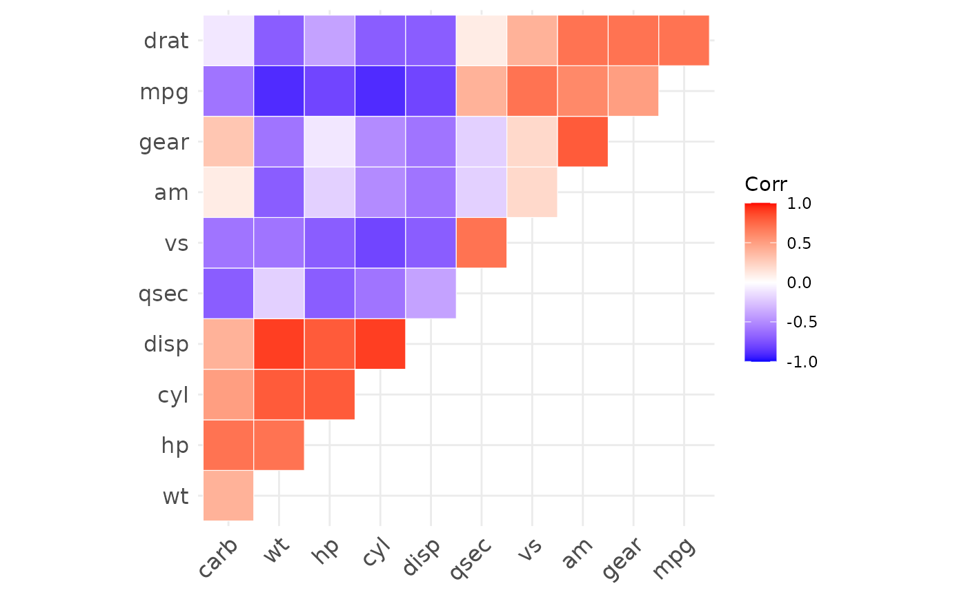
 # Get the upeper triangle
ggcorrplot(corr,
hc.order = TRUE, type = "upper",
outline.color = "white"
)
# Get the upeper triangle
ggcorrplot(corr,
hc.order = TRUE, type = "upper",
outline.color = "white"
)
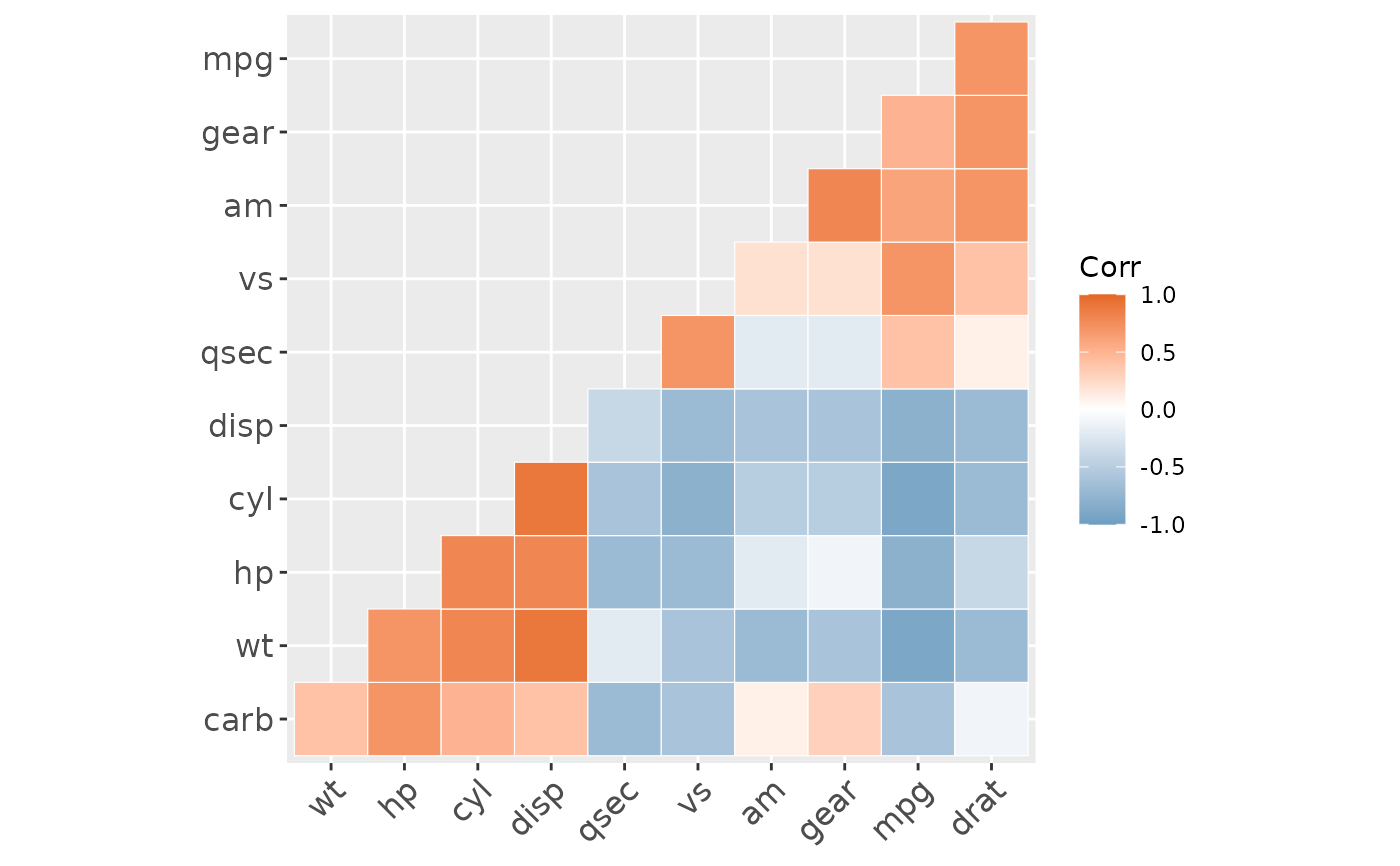
 # Change colors and theme
# --------------------------------
# Argument colors
ggcorrplot(corr,
hc.order = TRUE, type = "lower",
outline.color = "white",
ggtheme = ggplot2::theme_gray,
colors = c("#6D9EC1", "white", "#E46726")
)
# Change colors and theme
# --------------------------------
# Argument colors
ggcorrplot(corr,
hc.order = TRUE, type = "lower",
outline.color = "white",
ggtheme = ggplot2::theme_gray,
colors = c("#6D9EC1", "white", "#E46726")
)
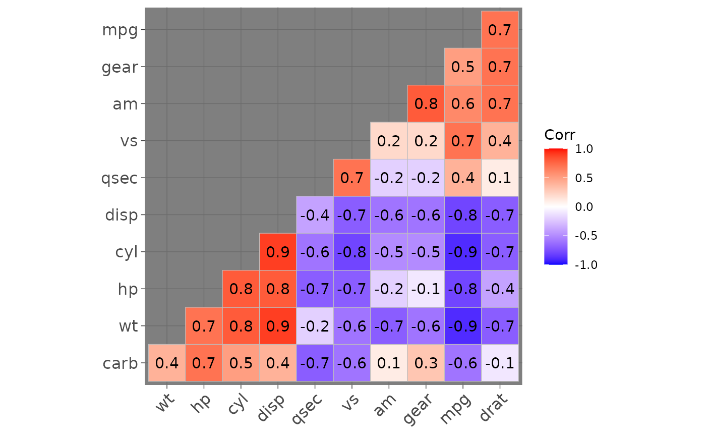
 # Add correlation coefficients
# --------------------------------
# argument lab = TRUE
ggcorrplot(corr,
hc.order = TRUE, type = "lower",
lab = TRUE,
ggtheme = ggplot2::theme_dark(),
)
# Add correlation coefficients
# --------------------------------
# argument lab = TRUE
ggcorrplot(corr,
hc.order = TRUE, type = "lower",
lab = TRUE,
ggtheme = ggplot2::theme_dark(),
)
 # Add correlation significance level
# --------------------------------
# Argument p.mat
# Barring the no significant coefficient
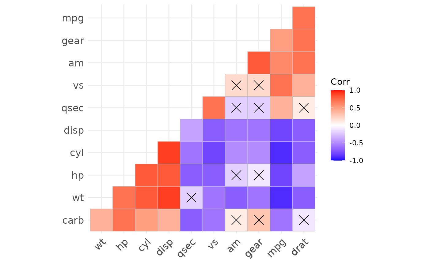
ggcorrplot(corr,
hc.order = TRUE,
type = "lower", p.mat = p.mat
)
# Add correlation significance level
# --------------------------------
# Argument p.mat
# Barring the no significant coefficient
ggcorrplot(corr,
hc.order = TRUE,
type = "lower", p.mat = p.mat
)
 # Leave blank on no significant coefficient
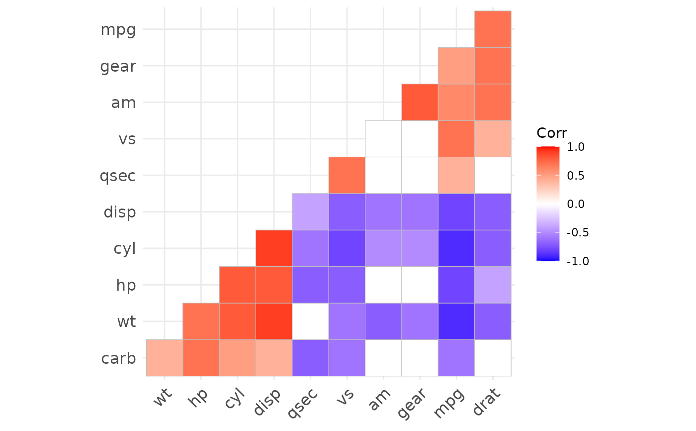
ggcorrplot(corr,
p.mat = p.mat, hc.order = TRUE,
type = "lower", insig = "blank"
)
# Leave blank on no significant coefficient
ggcorrplot(corr,
p.mat = p.mat, hc.order = TRUE,
type = "lower", insig = "blank"
)
 # Changing number of digits for correlation coeffcient
# --------------------------------
ggcorrplot(cor(mtcars),
type = "lower",
insig = "blank",
lab = TRUE,
digits = 3
)
# Changing number of digits for correlation coeffcient
# --------------------------------
ggcorrplot(cor(mtcars),
type = "lower",
insig = "blank",
lab = TRUE,
digits = 3
)