Fitted theoretical density

Estimates the parameters of a given distribution and evaluates the probability density function with these parameters. This can be useful for comparing histograms or kernel density estimates against a theoretical distribution.

stat_theodensity(
  mapping = NULL,
  data = NULL,
  geom = "line",
  position = "identity",
  ...,
  distri = "norm",
  n = 512,
  fix.arg = NULL,
  start.arg = NULL,
  na.rm = TRUE,
  show.legend = NA,
  inherit.aes = TRUE
)

Arguments

mapping

Set of aesthetic mappings created by aes(). If specified and inherit.aes = TRUE (the default), it is combined with the default mapping at the top level of the plot. You must supply mapping if there is no plot mapping.

data

The data to be displayed in this layer. There are three options:

If NULL, the default, the data is inherited from the plot data as specified in the call to ggplot().

A data.frame, or other object, will override the plot data. All objects will be fortified to produce a data frame. See fortify() for which variables will be created.

A function will be called with a single argument, the plot data. The return value must be a data.frame, and will be used as the layer data. A function can be created from a formula (e.g. ~ head(.x, 10)).

geom

Use to override the default geom for stat_theodensity.

position

A position adjustment to use on the data for this layer. This can be used in various ways, including to prevent overplotting and improving the display. The position argument accepts the following:

The result of calling a position function, such as position_jitter(). This method allows for passing extra arguments to the position.
A string naming the position adjustment. To give the position as a string, strip the function name of the position_ prefix. For example, to use position_jitter(), give the position as "jitter".
For more information and other ways to specify the position, see the layer position documentation.

...

Other arguments passed on to layer()'s params argument. These arguments broadly fall into one of 4 categories below. Notably, further arguments to the position argument, or aesthetics that are required can not be passed through .... Unknown arguments that are not part of the 4 categories below are ignored.

Static aesthetics that are not mapped to a scale, but are at a fixed value and apply to the layer as a whole. For example, colour = "red" or linewidth = 3. The geom's documentation has an Aesthetics section that lists the available options. The 'required' aesthetics cannot be passed on to the params. Please note that while passing unmapped aesthetics as vectors is technically possible, the order and required length is not guaranteed to be parallel to the input data.
When constructing a layer using a stat_*() function, the ... argument can be used to pass on parameters to the geom part of the layer. An example of this is stat_density(geom = "area", outline.type = "both"). The geom's documentation lists which parameters it can accept.
Inversely, when constructing a layer using a geom_*() function, the ... argument can be used to pass on parameters to the stat part of the layer. An example of this is geom_area(stat = "density", adjust = 0.5). The stat's documentation lists which parameters it can accept.
The key_glyph argument of layer() may also be passed on through .... This can be one of the functions described as key glyphs, to change the display of the layer in the legend.

distri

A character of length 1 naming a distribution without prefix. See details.

n

An integer of length 1 with the number of equally spaced points at which the density function is evaluated. Ignored if distribution is discrete.

fix.arg

An optional named list giving values of fixed parameters of the named distribution. Parameters with fixed value are not estimated by maximum likelihood procedures.

start.arg

A named list giving initial values of parameters for the named distribution. This argument may be omitted (default) for some distributions for which reasonable starting values are computed.

na.rm

If FALSE, the default, missing values are removed with a warning. If TRUE, missing values are silently removed.

show.legend

logical. Should this layer be included in the legends? NA, the default, includes if any aesthetics are mapped. FALSE never includes, and TRUE always includes. It can also be a named logical vector to finely select the aesthetics to display.

inherit.aes

If FALSE, overrides the default aesthetics, rather than combining with them. This is most useful for helper functions that define both data and aesthetics and shouldn't inherit behaviour from the default plot specification, e.g. borders().

Value

A Layer ggproto object.

Details

Valid distri arguments are the names of distributions for which there exists a density function. The names should be given without a prefix (typically 'd', 'r', 'q' and 'r'). For example: "norm" for the normal distribution and "nbinom" for the negative binomial distribution. Take a look at distributions() in the stats package for an overview.

There are a couple of distribution for which there exist no reasonable starting values, such as the Student t-distribution and the F-distribution. In these cases, it would probably be wise to provide reasonable starting values as a named list to the start.arg argument. When estimating a binomial distribution, it would be best to supply the size to the fix.arg argument.

By default, the y values are such that the integral of the distribution is 1, which scales well with the defaults of kernel density estimates. When comparing distributions with absolute count histograms, a sensible choice for aesthetic mapping would be aes(y = stat(count) * binwidth), wherein binwidth is matched with the bin width of the histogram.

For discrete distributions, the input data are expected to be integers, or doubles that can be divided by 1 without remainders.

Parameters are estimated using the fitdistrplus::fitdist() function in the fitdistrplus package using maximum likelihood estimation. Hypergeometric and multinomial distributions from the stats package are not supported.

Computed variables

density: probability density
count: density * number of observations - useful for comparing to histograms
scaled: density scaled to a maximum of 1

Examples

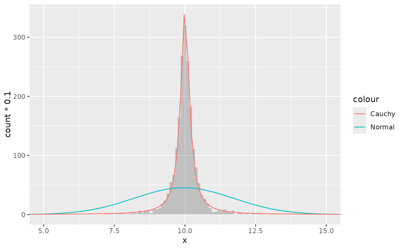
# A mixture of normal distributions where the standard deviation is
# inverse gamma distributed resembles a cauchy distribution.
x <- rnorm(2000, 10, 1/rgamma(2000, 2, 0.5))
df <- data.frame(x = x)

ggplot(df, aes(x)) +
  geom_histogram(binwidth = 0.1,
                 alpha = 0.3, position = "identity") +
  stat_theodensity(aes(y = stat(count) * 0.1, colour = "Normal"),
                   distri = "norm", geom = "line") +
  stat_theodensity(aes(y = stat(count) * 0.1, colour = "Cauchy"),
                   distri = "cauchy", geom = "line") +
  coord_cartesian(xlim = c(5, 15))
#> Warning: `stat(count)` was deprecated in ggplot2 3.4.0.
#> ℹ Please use `after_stat(count)` instead.


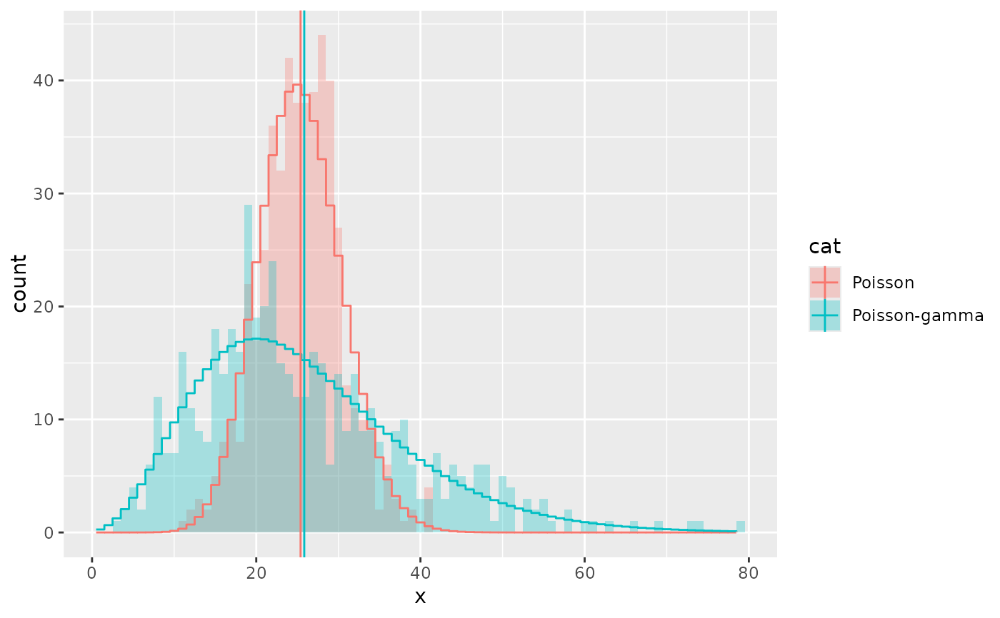
# A negative binomial can be understood as a Poisson-gamma mixture
df <- data.frame(x = c(rpois(500, 25),
                       rpois(500, rgamma(500, 5, 0.2))),
                 cat = rep(c("Poisson", "Poisson-gamma"), each = 500))

ggplot(df, aes(x)) +
  geom_histogram(binwidth = 1, aes(fill = cat),
                 alpha = 0.3, position = "identity") +
  stat_theodensity(aes(y = stat(count), colour = cat), distri = "nbinom",
                   geom = "step", position = position_nudge(x = -0.5)) +
  stat_summary(aes(y = x, colour = cat, x = 1),
               fun.data = function(x){data.frame(xintercept = mean(x))},
               geom = "vline")

Arguments

Value

Details

Computed variables

See also

Examples