Polar coordinates

The polar coordinate system is most commonly used for pie charts, which are a stacked bar chart in polar coordinates.
: coord_polar() has been in favour of coord_radial().

coord_polar(theta = "x", start = 0, direction = 1, clip = "on")

coord_radial(
  theta = "x",
  start = 0,
  end = NULL,
  thetalim = NULL,
  rlim = NULL,
  expand = TRUE,
  direction = deprecated(),
  clip = "off",
  r.axis.inside = NULL,
  rotate.angle = FALSE,
  inner.radius = 0,
  reverse = "none",
  r_axis_inside = deprecated(),
  rotate_angle = deprecated()
)

Arguments

theta

variable to map angle to (x or y)

start

Offset of starting point from 12 o'clock in radians. Offset is applied clockwise or anticlockwise depending on value of direction.

direction

1, clockwise; -1, anticlockwise

clip

Should drawing be clipped to the extent of the plot panel? A setting of "on" (the default) means yes, and a setting of "off" means no. For details, please see coord_cartesian().

end

Position from 12 o'clock in radians where plot ends, to allow for partial polar coordinates. The default, NULL, is set to start + 2 * pi.

thetalim, rlim

Limits for the theta and r axes.

expand

If TRUE, the default, adds a small expansion factor to the limits to prevent overlap between data and axes. If FALSE, limits are taken directly from the scale.

r.axis.inside

One of the following:

NULL (default) places the axis next to the panel if start and end arguments form a full circle and inside the panel otherwise.
TRUE to place the radius axis inside the panel.
FALSE to place the radius axis next to the panel.
A numeric value, setting a theta axis value at which the axis should be placed inside the panel. Can be given as a length 2 vector to control primary and secondary axis placement separately.

rotate.angle

If TRUE, transforms the angle aesthetic in data in accordance with the computed theta position. If FALSE (default), no such transformation is performed. Can be useful to rotate text geoms in alignment with the coordinates.

inner.radius

A numeric between 0 and 1 setting the size of a inner radius hole.

reverse

A string giving which directions to reverse. "none" (default) keep directions as is. "theta" reverses the angle and "r" reverses the radius. "thetar" reverses both the angle and the radius.

r_axis_inside, rotate_angle

Note

In coord_radial(), position guides can be defined by using guides(r = ..., theta = ..., r.sec = ..., theta.sec = ...). Note that these guides require r and theta as available aesthetics. The classic guide_axis() can be used for the r positions and guide_axis_theta() can be used for the theta positions. Using the theta.sec position is only sensible when inner.radius > 0.

Examples

# NOTE: Use these plots with caution - polar coordinates has
# major perceptual problems.  The main point of these examples is
# to demonstrate how these common plots can be described in the
# grammar.  Use with EXTREME caution.

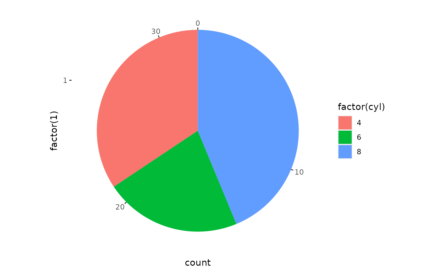
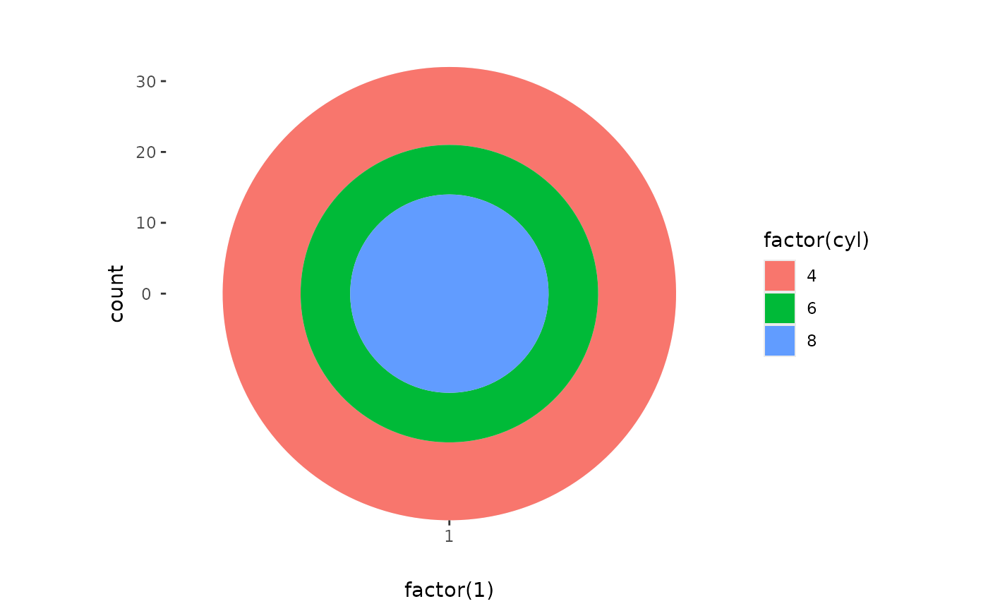
# A pie chart = stacked bar chart + polar coordinates
pie <- ggplot(mtcars, aes(x = factor(1), fill = factor(cyl))) +
 geom_bar(width = 1)
pie + coord_radial(theta = "y", expand = FALSE)


# \donttest{

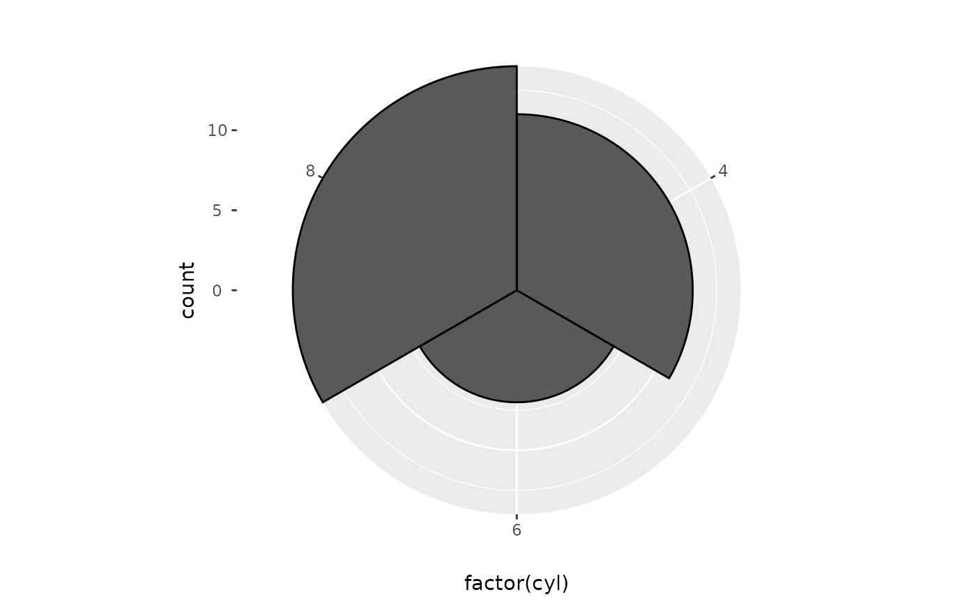
# A coxcomb plot = bar chart + polar coordinates
cxc <- ggplot(mtcars, aes(x = factor(cyl))) +
  geom_bar(width = 1, colour = "black")
cxc + coord_radial(expand = FALSE)

# A new type of plot?
cxc + coord_radial(theta = "y", expand = FALSE)


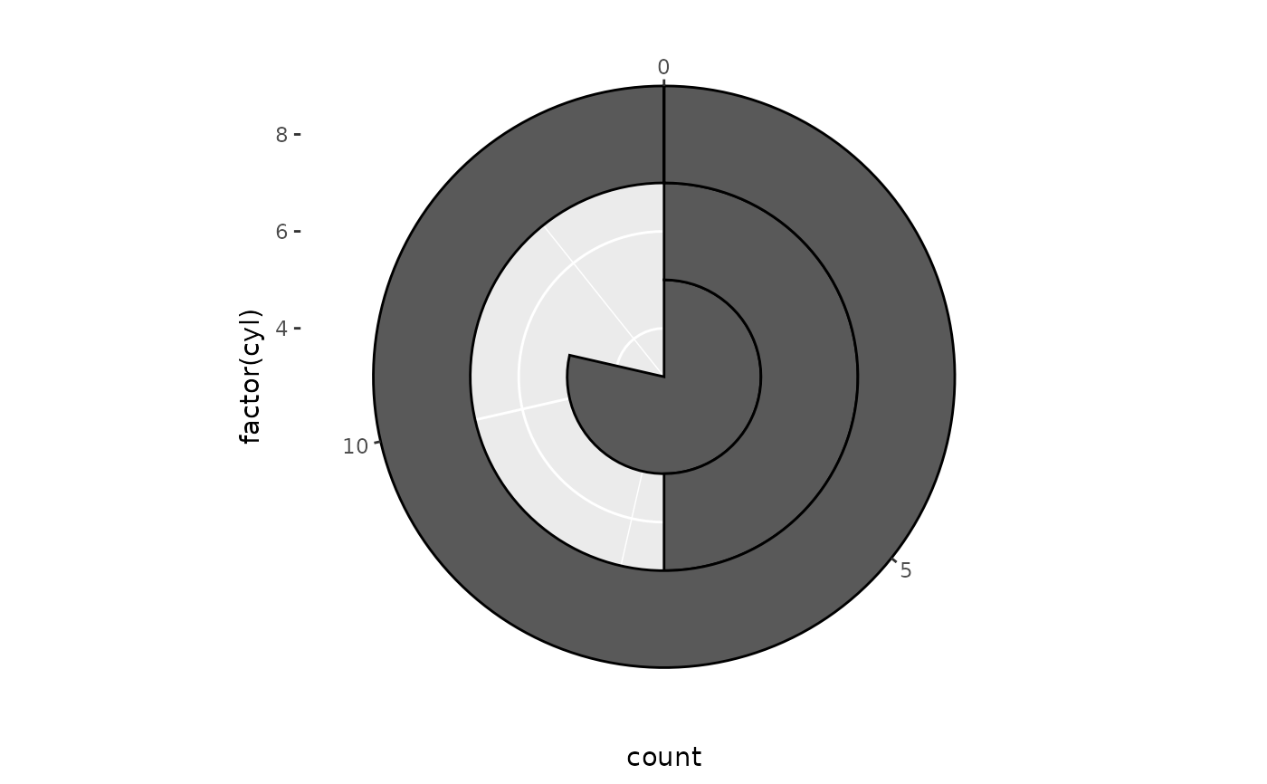# The bullseye chart
pie + coord_radial(expand = FALSE)


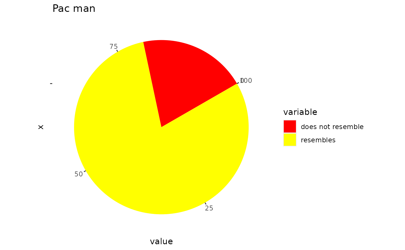
# Hadley's favourite pie chart
df <- data.frame(
  variable = c("does not resemble", "resembles"),
  value = c(20, 80)
)
ggplot(df, aes(x = "", y = value, fill = variable)) +
  geom_col(width = 1) +
  scale_fill_manual(values = c("red", "yellow")) +
  coord_radial("y", start = pi / 3, expand =  FALSE) +
  labs(title = "Pac man")


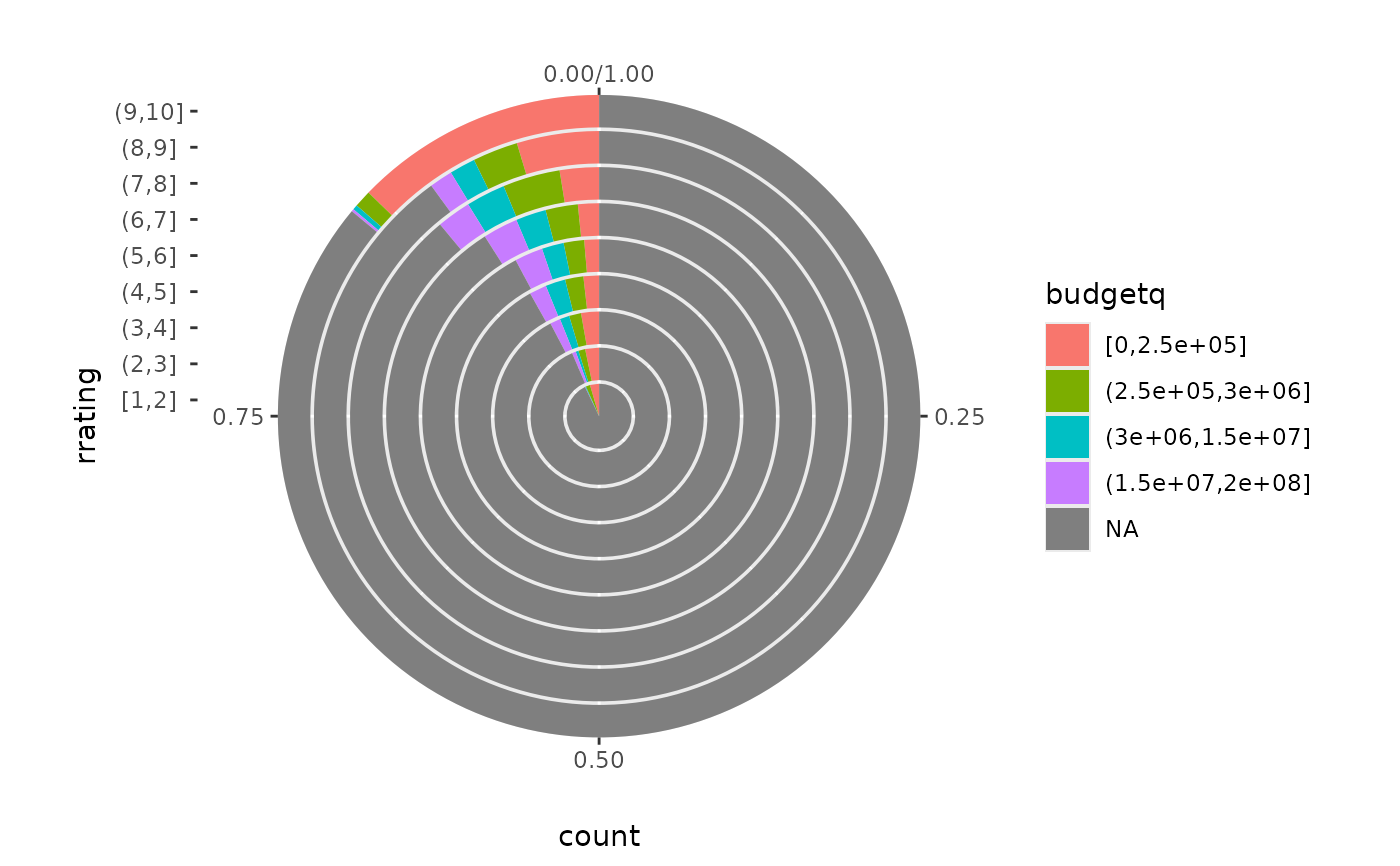
# Windrose + doughnut plot
if (require("ggplot2movies")) {
movies$rrating <- cut_interval(movies$rating, length = 1)
movies$budgetq <- cut_number(movies$budget, 4)

doh <- ggplot(movies, aes(x = rrating, fill = budgetq))

# Wind rose
doh + geom_bar(width = 1) + coord_radial(expand = FALSE)
# Race track plot
doh + geom_bar(width = 0.9, position = "fill") +
  coord_radial(theta = "y", expand = FALSE)
}
#> Loading required package: ggplot2movies

# }
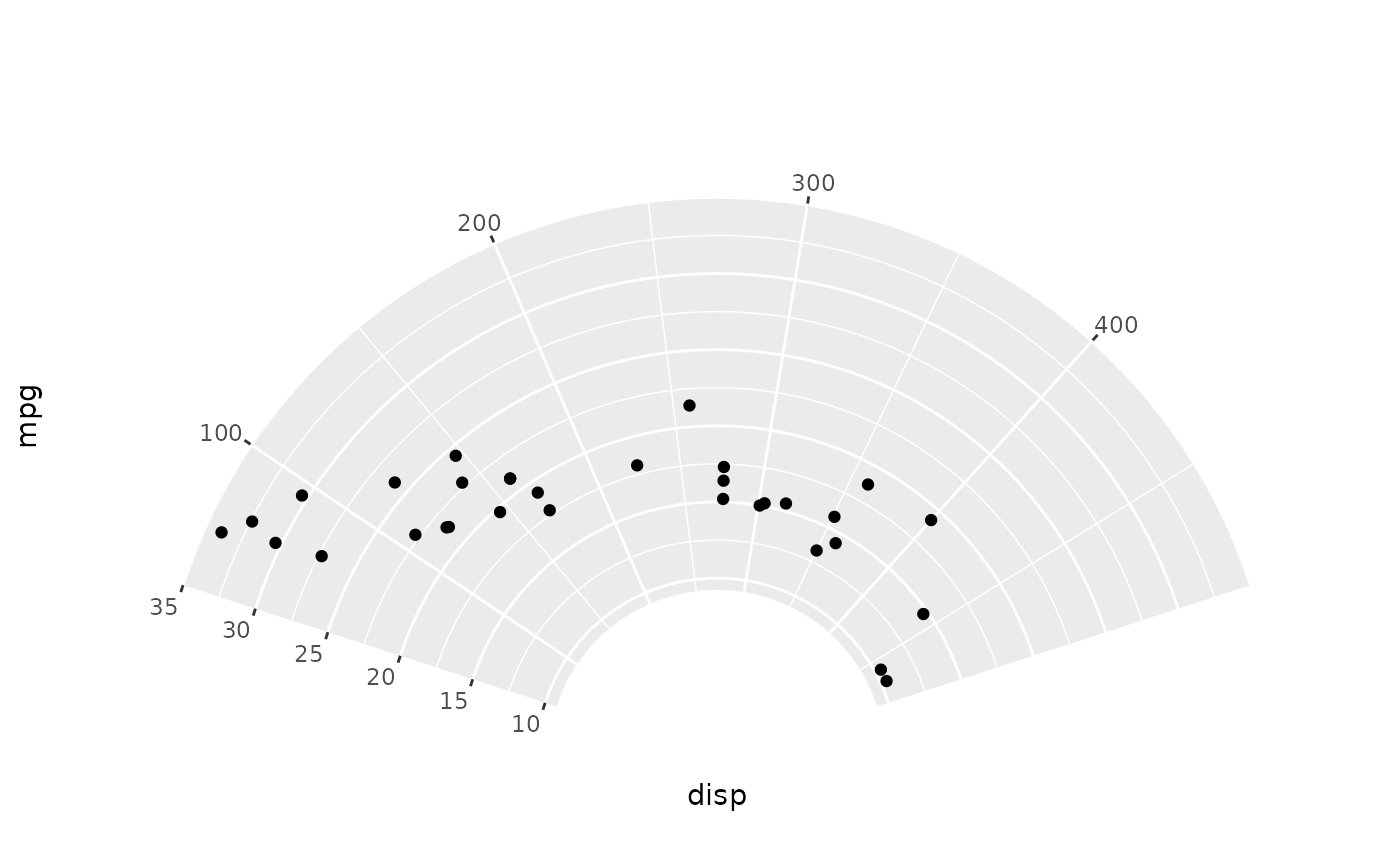
# A partial polar plot
ggplot(mtcars, aes(disp, mpg)) +
  geom_point() +
  coord_radial(start = -0.4 * pi, end = 0.4 * pi, inner.radius = 0.3)


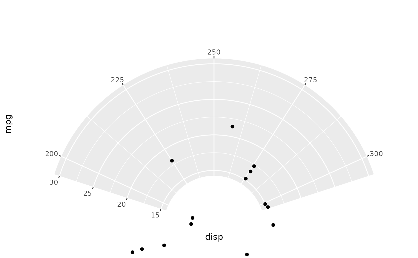
# Similar with coord_cartesian(), you can set limits.
ggplot(mtcars, aes(disp, mpg)) +
  geom_point() +
  coord_radial(
    start = -0.4 * pi,
    end = 0.4 * pi, inner.radius = 0.3,
    thetalim = c(200, 300),
    rlim = c(15, 30),
  )

Arguments

Note

See also

Examples