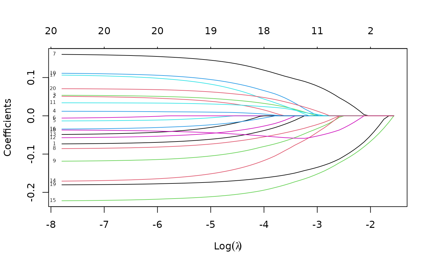
plot coefficients from a "glmnet" object

Produces a coefficient profile plot of the coefficient paths for a fitted "glmnet" object.

# S3 method for class 'glmnet'
plot(x, xvar = c("lambda", "norm", "dev"), label = FALSE, ...)

# S3 method for class 'mrelnet'
plot(
  x,
  xvar = c("lambda", "norm", "dev"),
  label = FALSE,
  type.coef = c("coef", "2norm"),
  ...
)

# S3 method for class 'multnet'
plot(
  x,
  xvar = c("lambda", "norm", "dev"),
  label = FALSE,
  type.coef = c("coef", "2norm"),
  ...
)

# S3 method for class 'relaxed'
plot(x, xvar = c("lambda", "dev"), label = FALSE, gamma = 1, ...)

Arguments

x: fitted "glmnet" model
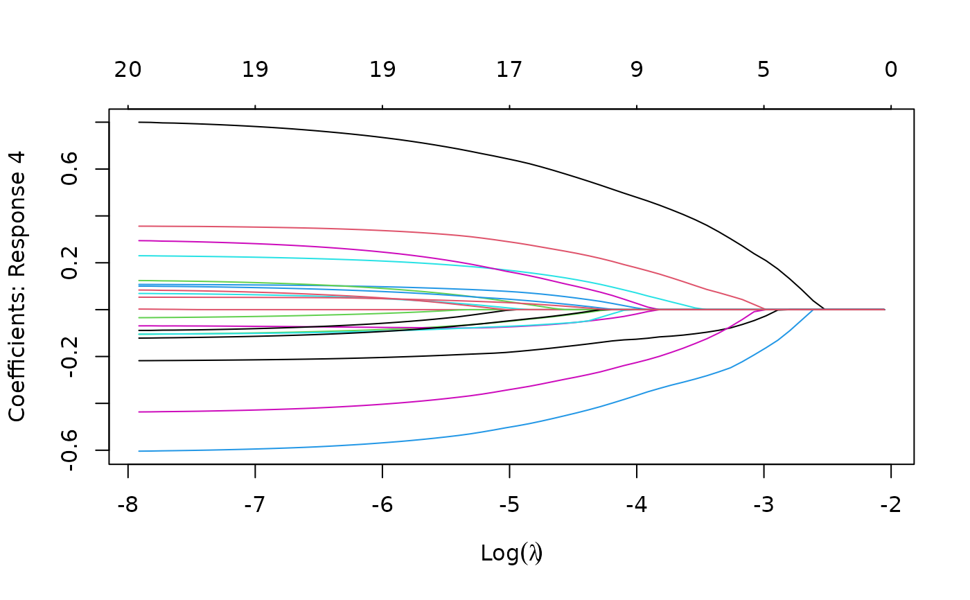
xvar: What is on the X-axis. "lambda" plots against the log-lambda sequence, "norm" against the L1-norm of the coefficients, and "dev" against the percent deviance explained. Warning: "norm" is the L1 norm of the coefficients on the glmnet object. There are many reasons why this might not be appropriate, such as automatic standardization, penalty factors, and values of alpha less than 1, which can lead to unusual looking plots.
label: If TRUE, label the curves with variable sequence numbers.
...: Other graphical parameters to plot
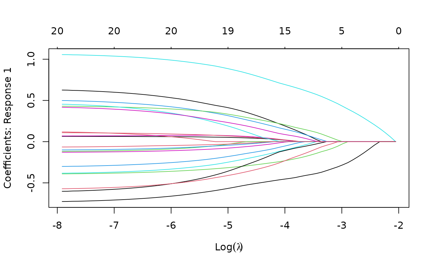
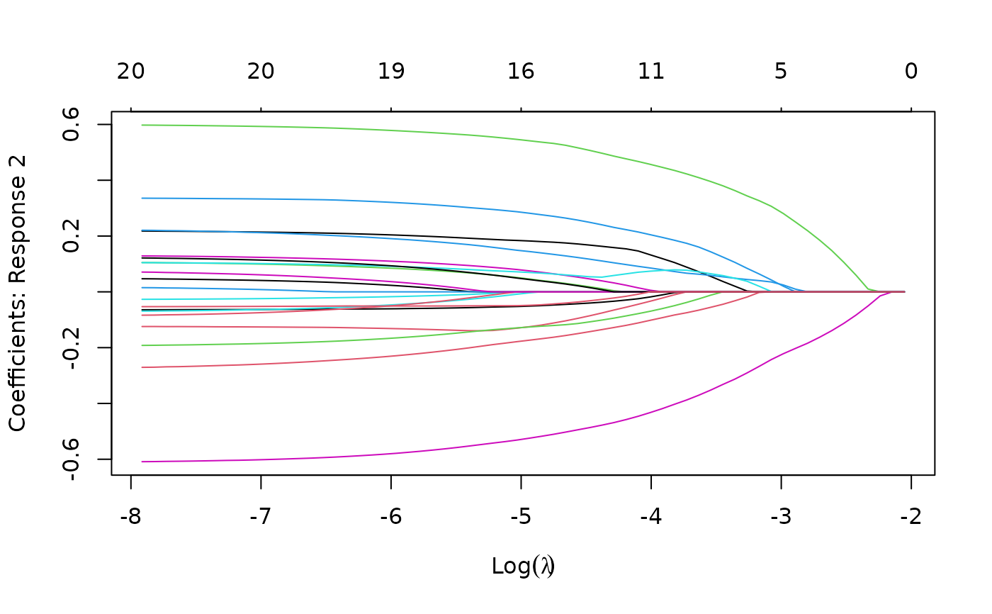
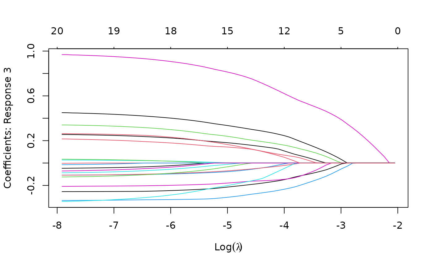
type.coef: If type.coef="2norm" then a single curve per variable, else if type.coef="coef", a coefficient plot per response
gamma: Value of the mixing parameter for a "relaxed" fit

Details

A coefficient profile plot is produced. If x is a multinomial model, a coefficient plot is produced for each class.

References

Friedman, J., Hastie, T. and Tibshirani, R. (2008) Regularization Paths for Generalized Linear Models via Coordinate Descent

Author

Jerome Friedman, Trevor Hastie and Rob Tibshirani
Maintainer: Trevor Hastie hastie@stanford.edu

Examples

x=matrix(rnorm(100*20),100,20)
y=rnorm(100)
g2=sample(1:2,100,replace=TRUE)
g4=sample(1:4,100,replace=TRUE)
fit1=glmnet(x,y)
plot(fit1)
plot(fit1,xvar="lambda",label=TRUE)

fit3=glmnet(x,g4,family="multinomial")
plot(fit3,pch=19)