Productivity and Quit Behavior of Western Electric Workers

Partially artificial data about quit behavior of Western Electric workers. (Western Electric was the manufacturing arm of the AT&T corporation during its glory days as a monopolist in the U.S. telephone industry.)

Usage

data("WECO")

Format

A data frame containing 683 observations on 7 variables.

output: productivity in first six months.
sex: factor indicating gender.
dex: score on a preemployment dexterity exam.
lex: years of education.
kwit: factor indicating whether the worker quit in the first six months.
tenure: duration of employment (see details).
censored: logical. Is the duration censored?

Details

The explanatory variables in this example are taken from the study of Klein et al. (1991), but the response variable was altered long ago to improve the didactic impact of the model as a class exercise. To this end, quit dates for each individual were generated according to a log Weibull proportional hazard model.

Source

Online supplements to Koenker (2006) and Koenker and Yoon (2009).

http://www.econ.uiuc.edu/~roger/research/links/links.html

References

Klein R, Spady R, Weiss A (1991). “Factors Affecting the Output and Quit Propensities of Production Workers.” The Review of Economic Studies, 58(5), 929–953.

Koenker R (2006). “Parametric Links for Binary Response.” R News, 6(4), 32–34.

Koenker R, Yoon J (2009). “Parametric Links for Binary Choice Models: A Fisherian-Bayesian Colloquy.” Journal of Econometrics, 152, 120–130.

Examples

# \donttest{
## WECO data
data("WECO", package = "glmx")
f <- kwit ~ sex + dex + poly(lex, 2, raw = TRUE)
## (raw = FALSE would be numerically more stable)

## Gosset model
gossbin <- function(nu) binomial(link = gosset(nu))
m1 <- glmx(f, data = WECO,
  family = gossbin, xstart = 0, xlink = "log")

## Pregibon model
pregibin <- function(shape) binomial(link = pregibon(shape[1], shape[2]))
m2 <- glmx(f, data = WECO,
  family = pregibin, xstart = c(0, 0), xlink = "identity")

## Probit/logit/cauchit models
m3 <- lapply(c("probit", "logit", "cauchit"), function(nam)
  glm(f, data = WECO, family = binomial(link = nam)))

## Probit/cauchit vs. Gosset
if(require("lmtest")) {
lrtest(m3[[1]], m1)
lrtest(m3[[3]], m1)

## Logit vs. Pregibon
lrtest(m3[[2]], m2)
}
#> Warning: original model was of class "glm", updated model is of class "glmx"
#> Warning: original model was of class "glm", updated model is of class "glmx"
#> Warning: original model was of class "glm", updated model is of class "glmx"
#> Likelihood ratio test
#> 
#> Model 1: kwit ~ sex + dex + poly(lex, 2, raw = TRUE)
#> Model 2: f
#>   #Df  LogLik Df  Chisq Pr(>Chisq)    
#> 1   5 -368.33                         
#> 2   7 -360.91  2 14.845  0.0005976 ***
#> ---
#> Signif. codes:  0 ‘***’ 0.001 ‘**’ 0.01 ‘*’ 0.05 ‘.’ 0.1 ‘ ’ 1

## Table 1
tab1 <- sapply(c(m3, list(m1)), function(obj)
  c(head(coef(obj), 5), AIC(obj)))
colnames(tab1) <- c("Probit", "Logit", "Cauchit", "Gosset")
rownames(tab1)[4:6] <- c("lex", "lex^2", "AIC")
tab1 <- round(t(tab1), digits = 3)
tab1
#>         (Intercept) sexmale    dex    lex lex^2     AIC
#> Probit        3.549   0.268 -0.053 -0.313 0.012 748.711
#> Logit         6.220   0.479 -0.094 -0.539 0.021 746.663
#> Cauchit       8.234   0.677 -0.125 -0.694 0.028 736.881
#> Gosset       20.364   1.675 -0.297 -1.730 0.069 734.409

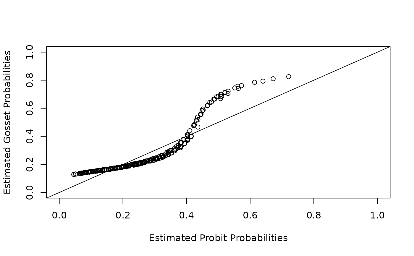
## Figure 4
plot(fitted(m3[[1]]), fitted(m1),
  xlim = c(0, 1), ylim = c(0, 1),
  xlab = "Estimated Probit Probabilities",
  ylab = "Estimated Gosset Probabilities")
abline(0, 1)

# }