This function simplifies the selection of relevant species in ordination diagrams. It works with result objects from the vegan package. The selection can be based upon cover abundances, frequency values and/or species fit to multivariate analysis (see Details).
The result is a vector of names of the selected species and can be used for the select argument in ordination plots.
ordiselect(
  matrix,
  ord,
  ablim = 1,
  fitlim = 1,
  choices = c(1, 2),
  freq = FALSE,
  na.rm = FALSE,
  method = "axes",
  env,
  p.max = 0.05
)
Arguments
- matrix
Community data, a matrix-like object with samples in rows and species in columns.
- ord
veganordination result object (e.g. fromdecorana,ccaormetaMDS).- ablim
Proportion of species with highest abundances to be displayed. Value between 0 and 1. Use negative sign for selection of lowest abundances, i.e. rarest species.
- fitlim
Proportion of species with best fit to be displayed. Value between 0 and 1.
- choices
Axes shown.
- freq
Whether to use cover abundances (= default) or frequencies of
matrix. IfTRUE, frequencies of species are used.- na.rm
Set to
TRUEif your ordination object contains NA (e.g. due to selection)- method
The species fit method:
"axes"(= default) or"factors". See details for methods.- env
Fitted environmental variables (result object of
envfit) formethod = "factors". Only factor variables are used.- p.max
Significance limit for variables used in
method = "factors".
Value
A vector of variable length containing the names of selected species from matrix.
Details
Two methods for species fit are implemented.
In
method = "factors", Euclidean distances between species and environmental variable centroids are calculated. Only factor variables are used fromenvfitoutput. The species with smallest distances, defined byfitlimargument as a threshold, will be filtered from the ordination result. Thep.maxargument allows selection of only significant variables, default isp.max = 0.05.
The species fit methods work well both in eigenvalue-based and in distance-based ordinations and provide good option of objective reduction of visible species in ordination plot for better interpretation issues.
If axes fit should be applied on distance-based ordination, species scores need to be calculated during the analysis, e.g. by selecting wascores = TRUE in metaMDS. It is mostly recommendable to combine the species fit limit with an abundance limit to avoid overinterpretation of rare species.
For the abundance limit, note that the final proportion of the selected species may be higher than the indicated proportion if there are identical values in the abundances.
For selection of least abundant (rarest) species you can use a negative sign, e.g. ablim = -0.3 for the 30 percent least abundant species.
If both limits are defined only species meeting both conditions are selected.
If no limit is defined for one of the arguments ablim, fitlim, all species are displayed.
The default for matrix input is a cover-abundance-matrix. This matrix should also be used for ordination.
Examples
## Calculate DCA
library(vegan)
#> Loading required package: permute
scheden.dca <- decorana(schedenveg)
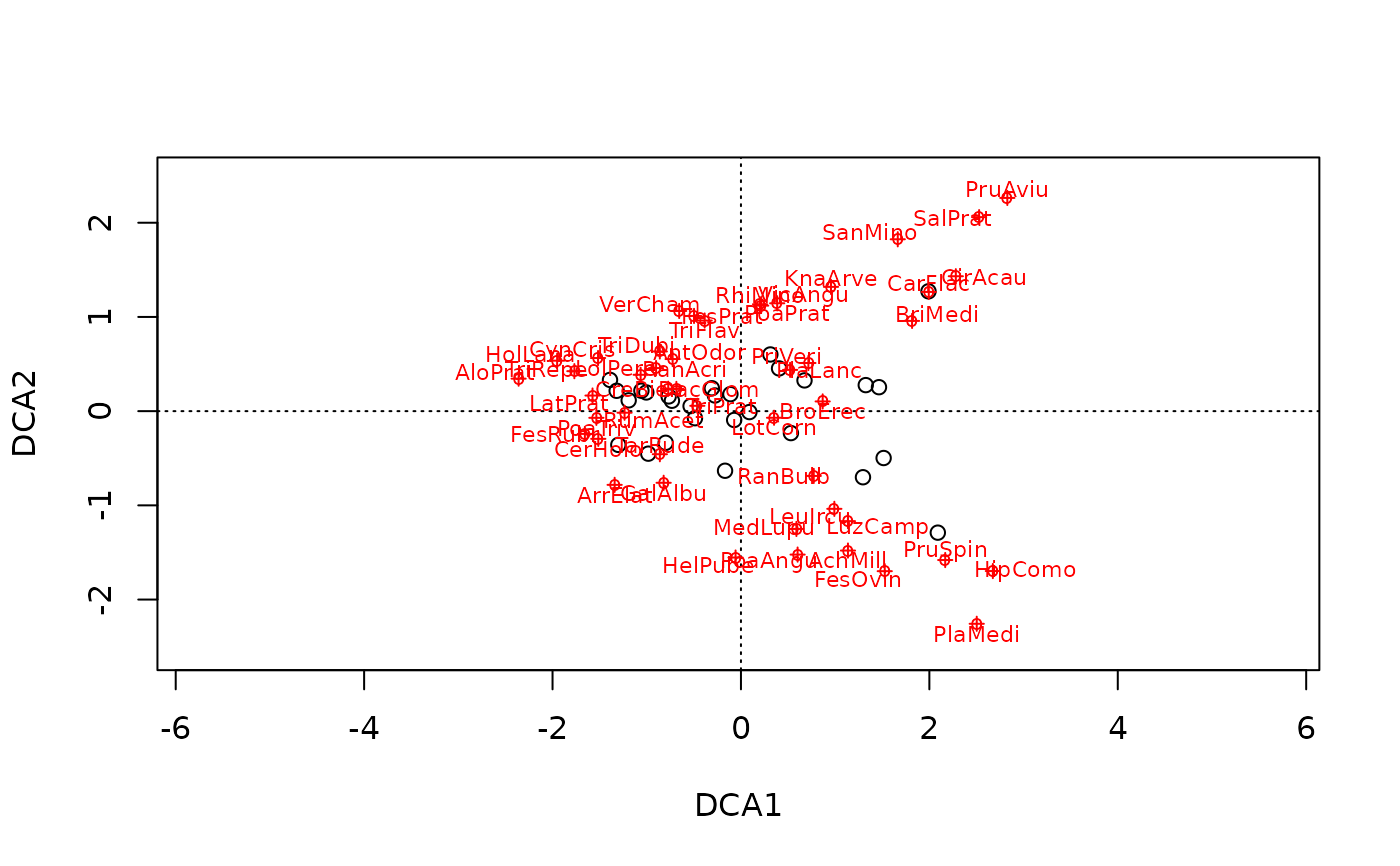
## Select the 30% most abundant species and call the result
limited <- ordiselect(schedenveg, scheden.dca, ablim = 0.3)
#> [1] "47 species selected (30.3% of total number of species)."
#> [1] "All species selected which belong to the 30% most abundant species."
limited
#> [1] "AchMill" "AloPrat" "AntOdor" "ArrElat" "BriMedi" "BroErec" "CarFlac"
#> [8] "CerHolo" "CirAcau" "CreBien" "CynCris" "DacGlom" "FesOvin" "FesPrat"
#> [15] "FesRubr" "GalAlbu" "HelPube" "HipComo" "HolLana" "KnaArve" "LatPrat"
#> [22] "LeuIrcu" "LolPere" "LotCorn" "LuzCamp" "MedLupu" "PlaLanc" "PlaMedi"
#> [29] "PoaAngu" "PoaPrat" "PoaTriv" "PriVeri" "PruAviu" "PruSpin" "RanAcri"
#> [36] "RanBulb" "RhiMino" "RumAcet" "SalPrat" "SanMino" "TarRude" "TriDubi"
#> [43] "TriPrat" "TriRepe" "TriFlav" "VerCham" "VicAngu"
# Use the result in plotting
plot(scheden.dca, display="n")
points(scheden.dca, display="sites")
points(scheden.dca, display="species",
select = limited, pch = 3, col = "red", cex = 0.7)
ordipointlabel(scheden.dca, display="species",
select = limited, col="red", cex = 0.7, add = TRUE)
 ## Select the 70% of the species with the best fit to the axes (highest species scores)
## AND belonging to the 30% most frequent species
limited <- ordiselect(schedenveg, scheden.dca, ablim = 0.3,
fitlim = 0.7, freq = TRUE)
#> [1] "28 species selected (18.1% of total number of species)."
#> [1] "All species selected which belong to the 30% most frequent species and to the 70% of species with the highest absolute axis scores."
## Select the 30% least frequent species and call the result
limited <- ordiselect(schedenveg, scheden.dca, ablim = -0.3, freq = TRUE)
#> [1] "50 species selected (32.3% of total number of species)."
#> [1] "All species selected which belong to the 30% least frequent species."
limited
#> [1] "AceCamp" "AjuGene" "AjuRept" "AntDioi" "AraThal" "AreSerp" "AstGlyc"
#> [8] "BetPend" "CalSepi" "CamGlom" "CenEryt" "CerArve" "CirArve" "CorAvel"
#> [15] "CraMono" "EupSpec" "FraVesc" "FraExce" "GalPumi" "GerMoll" "GeuUrba"
#> [22] "HelNumm" "HypMacu" "JunComm" "LeoAutu" "LuzMult" "LysNumm" "MedFalc"
#> [29] "OnoVici" "OphInse" "OrcMasc" "PinSpec" "PlaLaet" "PotAnse" "PotRept"
#> [36] "PruGran" "RanSpec" "RosCani" "RubFrut" "RubIdae" "RumObtu" "SedSexa"
#> [43] "SilPusi" "SteGram" "TarEryt" "TriCamp" "UrtDioi" "ValCari" "VerHede"
#> [50] "VibOpul"
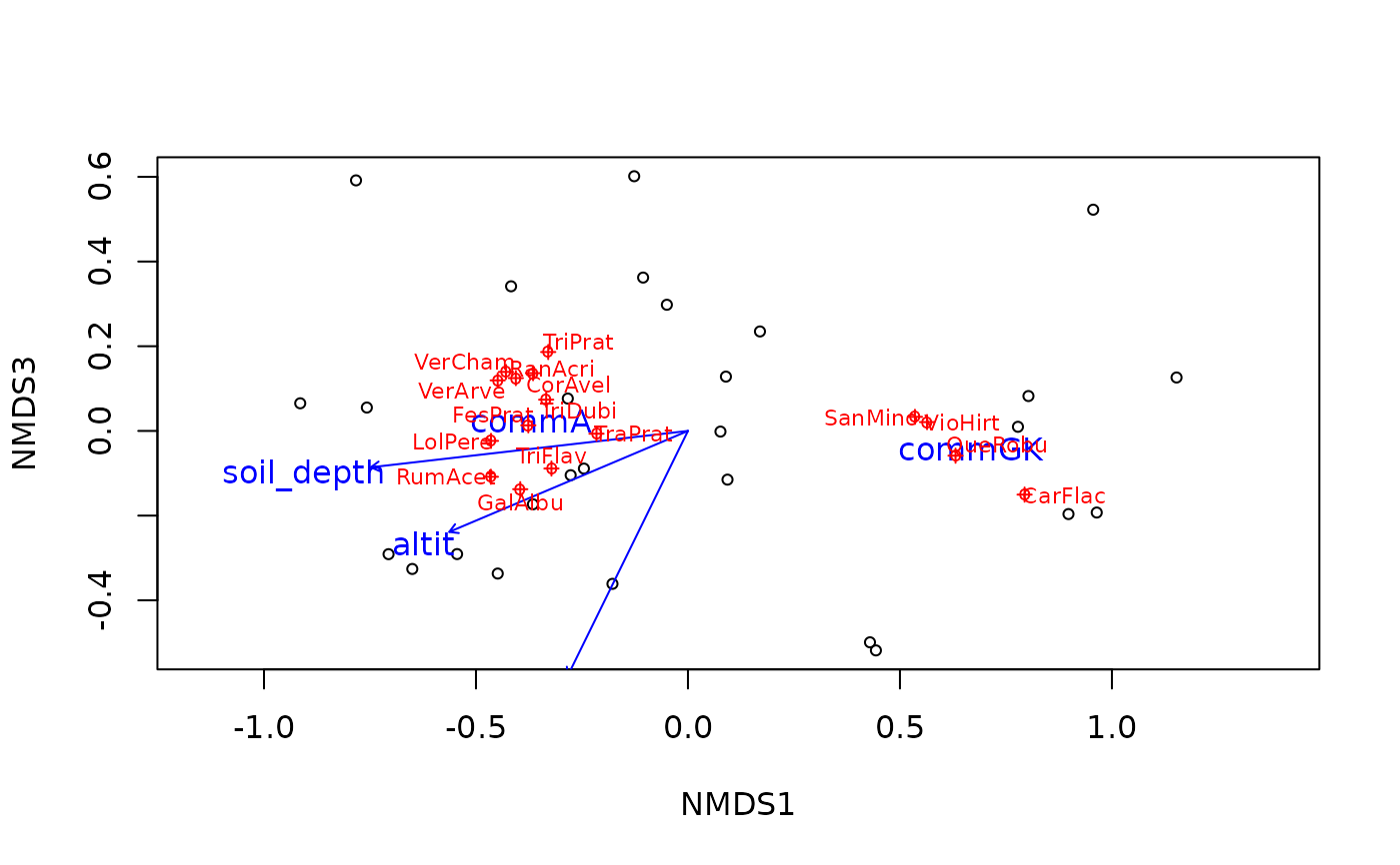
## Select the 20% of species with the best fit to community assignment
## AND belonging to the 50% most abundant
## in NDMS for axes 1 & 3
nmds <- metaMDS(schedenveg, k = 3) # run NMDS
#> Wisconsin double standardization
#> Run 0 stress 0.1247262
#> Run 1 stress 0.1285876
#> Run 2 stress 0.1247261
#> ... New best solution
#> ... Procrustes: rmse 5.967975e-05 max resid 0.0002276744
#> ... Similar to previous best
#> Run 3 stress 0.1284819
#> Run 4 stress 0.1247264
#> ... Procrustes: rmse 0.0002149998 max resid 0.0008324442
#> ... Similar to previous best
#> Run 5 stress 0.1247265
#> ... Procrustes: rmse 0.001033769 max resid 0.003284621
#> ... Similar to previous best
#> Run 6 stress 0.1247264
#> ... Procrustes: rmse 0.0001427812 max resid 0.0005342734
#> ... Similar to previous best
#> Run 7 stress 0.1328268
#> Run 8 stress 0.1343169
#> Run 9 stress 0.1277863
#> Run 10 stress 0.1247259
#> ... New best solution
#> ... Procrustes: rmse 0.0001572774 max resid 0.0003981064
#> ... Similar to previous best
#> Run 11 stress 0.1285803
#> Run 12 stress 0.1334434
#> Run 13 stress 0.1341683
#> Run 14 stress 0.1295195
#> Run 15 stress 0.1247262
#> ... Procrustes: rmse 0.0001852979 max resid 0.0005965968
#> ... Similar to previous best
#> Run 16 stress 0.1247263
#> ... Procrustes: rmse 0.000234452 max resid 0.0007883496
#> ... Similar to previous best
#> Run 17 stress 0.1320818
#> Run 18 stress 0.1285807
#> Run 19 stress 0.1277861
#> Run 20 stress 0.1289558
#> *** Best solution repeated 3 times
env13 <- envfit(nmds, schedenenv, choices = c(1, 3))
limited13 <- ordiselect(schedenveg, nmds, method = "factors",
fitlim = 0.1, ablim = 1,
choices = c(1,3), env = env13)
#> [1] "16 species selected (10.3% of total number of species)."
#> [1] "All species selected which belong to the 10% of species with the smallest distance to variable centroids."
# Use the result in plotting
plot(nmds, display="sites", choices = c(1, 3))
plot(env13, p.max = 0.05)
points(nmds, display="species", choices = c(1,3),
select = limited13, pch = 3, col="red", cex=0.7)
ordipointlabel(nmds, display="species", choices = c(1,3),
select = limited13, col="red", cex=0.7, add = TRUE)
## Select the 70% of the species with the best fit to the axes (highest species scores)
## AND belonging to the 30% most frequent species
limited <- ordiselect(schedenveg, scheden.dca, ablim = 0.3,
fitlim = 0.7, freq = TRUE)
#> [1] "28 species selected (18.1% of total number of species)."
#> [1] "All species selected which belong to the 30% most frequent species and to the 70% of species with the highest absolute axis scores."
## Select the 30% least frequent species and call the result
limited <- ordiselect(schedenveg, scheden.dca, ablim = -0.3, freq = TRUE)
#> [1] "50 species selected (32.3% of total number of species)."
#> [1] "All species selected which belong to the 30% least frequent species."
limited
#> [1] "AceCamp" "AjuGene" "AjuRept" "AntDioi" "AraThal" "AreSerp" "AstGlyc"
#> [8] "BetPend" "CalSepi" "CamGlom" "CenEryt" "CerArve" "CirArve" "CorAvel"
#> [15] "CraMono" "EupSpec" "FraVesc" "FraExce" "GalPumi" "GerMoll" "GeuUrba"
#> [22] "HelNumm" "HypMacu" "JunComm" "LeoAutu" "LuzMult" "LysNumm" "MedFalc"
#> [29] "OnoVici" "OphInse" "OrcMasc" "PinSpec" "PlaLaet" "PotAnse" "PotRept"
#> [36] "PruGran" "RanSpec" "RosCani" "RubFrut" "RubIdae" "RumObtu" "SedSexa"
#> [43] "SilPusi" "SteGram" "TarEryt" "TriCamp" "UrtDioi" "ValCari" "VerHede"
#> [50] "VibOpul"
## Select the 20% of species with the best fit to community assignment
## AND belonging to the 50% most abundant
## in NDMS for axes 1 & 3
nmds <- metaMDS(schedenveg, k = 3) # run NMDS
#> Wisconsin double standardization
#> Run 0 stress 0.1247262
#> Run 1 stress 0.1285876
#> Run 2 stress 0.1247261
#> ... New best solution
#> ... Procrustes: rmse 5.967975e-05 max resid 0.0002276744
#> ... Similar to previous best
#> Run 3 stress 0.1284819
#> Run 4 stress 0.1247264
#> ... Procrustes: rmse 0.0002149998 max resid 0.0008324442
#> ... Similar to previous best
#> Run 5 stress 0.1247265
#> ... Procrustes: rmse 0.001033769 max resid 0.003284621
#> ... Similar to previous best
#> Run 6 stress 0.1247264
#> ... Procrustes: rmse 0.0001427812 max resid 0.0005342734
#> ... Similar to previous best
#> Run 7 stress 0.1328268
#> Run 8 stress 0.1343169
#> Run 9 stress 0.1277863
#> Run 10 stress 0.1247259
#> ... New best solution
#> ... Procrustes: rmse 0.0001572774 max resid 0.0003981064
#> ... Similar to previous best
#> Run 11 stress 0.1285803
#> Run 12 stress 0.1334434
#> Run 13 stress 0.1341683
#> Run 14 stress 0.1295195
#> Run 15 stress 0.1247262
#> ... Procrustes: rmse 0.0001852979 max resid 0.0005965968
#> ... Similar to previous best
#> Run 16 stress 0.1247263
#> ... Procrustes: rmse 0.000234452 max resid 0.0007883496
#> ... Similar to previous best
#> Run 17 stress 0.1320818
#> Run 18 stress 0.1285807
#> Run 19 stress 0.1277861
#> Run 20 stress 0.1289558
#> *** Best solution repeated 3 times
env13 <- envfit(nmds, schedenenv, choices = c(1, 3))
limited13 <- ordiselect(schedenveg, nmds, method = "factors",
fitlim = 0.1, ablim = 1,
choices = c(1,3), env = env13)
#> [1] "16 species selected (10.3% of total number of species)."
#> [1] "All species selected which belong to the 10% of species with the smallest distance to variable centroids."
# Use the result in plotting
plot(nmds, display="sites", choices = c(1, 3))
plot(env13, p.max = 0.05)
points(nmds, display="species", choices = c(1,3),
select = limited13, pch = 3, col="red", cex=0.7)
ordipointlabel(nmds, display="species", choices = c(1,3),
select = limited13, col="red", cex=0.7, add = TRUE)