This function fits species response curves to visualize species responses to environmental gradients or ordination axes. It is based on Logistic Regression (binomial family) using Generalized Linear Models (GLMs) or Generalized Additive Models (GAMs) with integrated smoothness estimation. The function can draw response curves for single or multiple species.
specresponse(
  species,
  var,
  main,
  xlab,
  model = "auto",
  method = "env",
  axis = 1,
  points = FALSE,
  bw = FALSE,
  lwd = NULL,
  na.action = na.omit
)
Arguments
- species
Species data (either a community matrix object with samples in rows and species in columns - response curves are drawn for all (selected) columns; or a single vector containing species abundances per plot).
- var
Vector containing environmental variable (per plot) OR
veganordination result object ifmethod = "ord".- main
Optional: Main title.
- xlab
Optional: Label of x-axis.
- model
Defining the assumed species response: Default
model = "auto"selects the model automatically based on AIC. Other methods aremodel = "linear"(linear response),model = "unimodal"(unimodal response),model = "bimodal"(bimodal response) andmodel = "gam"(using GAM with regression smoother).- method
Method defining the type of variable. Default
method = "env"fits a response curve to environmental variables. Alternativelymethod = "ord"fits a response along ordination axes.- axis
Ordination axis (only if
method = "ord").- points
If set on
TRUEthe species occurrences are shown as transparent points (the darker the point the more samples at this x-value). To avoid overlapping they are shown with vertical offset when multiple species are displayed.- bw
If set on
TRUEthe lines will be drawn in black/white with different line types instead of colors.- lwd
Optional: Graphical parameter defining the line width.
- na.action
Optional: a function which indicates what should happen when the data contain NAs. The default is 'na.omit' (removes incomplete cases).
Value
Returns an (invisible) list with results for all calculated models. This list can be stored by assigning the result. For each model short information on type, parameters, explained deviance and corresponding p-value (based on chi-squared test) are printed.
Details
For response curves based on environmental gradients the argument var takes a single vector containing the variable corresponding to the species abundances.
For a response to ordination axis (method = "ord") the argument var requires a vegan ordination result object (e.g. from decorana, cca or metaMDS).
First axis is used as default.
By default the response curves are drawn with automatic GLM model selection based on AIC out of GLMs with 1 - 3 polynomial degrees (thus excluding bimodal responses which must be manually defined). The GAM model is more flexible and chooses automatically between an upper limit of 3 - 6 degrees of freedom for the regression smoother.
Available information about species is reduced to presence-absence as species abundances can contain much noise (being affected by complex factors) and the results of Logistic Regression are easier to interpret showing the "probabilities of occurrence". Be aware that response curves are only a simplification of reality (model) and their shape is strongly dependent on the available dataset.
Examples
## Draw species response curve for one species on environmental variable
## with points of occurrences
specresponse(schedenveg$ArrElat, schedenenv$soil_depth, points = TRUE)
 #> [1] "GLM with 2 degrees fitted for schedenveg$ArrElat. Deviance explained: 14%, p-value = 0.11."
## Draw species response curve on environmental variable with custom labels
specresponse(schedenveg$ArrElat, schedenenv$soil_depth, points = TRUE,
main = "Arrhenatherum elatius", xlab = "Soil depth")
#> [1] "GLM with 2 degrees fitted for schedenveg$ArrElat. Deviance explained: 14%, p-value = 0.11."
## Draw species response curve on environmental variable with custom labels
specresponse(schedenveg$ArrElat, schedenenv$soil_depth, points = TRUE,
main = "Arrhenatherum elatius", xlab = "Soil depth")
 #> [1] "GLM with 2 degrees fitted for schedenveg$ArrElat. Deviance explained: 14%, p-value = 0.11."
## Draw species response curve on ordination axes
## First calculate DCA
library(vegan)
scheden.dca <- decorana(schedenveg)
# Using a linear model on first axis
specresponse(schedenveg$ArrElat, scheden.dca, method = "ord", model = "linear")
#> [1] "GLM with 2 degrees fitted for schedenveg$ArrElat. Deviance explained: 14%, p-value = 0.11."
## Draw species response curve on ordination axes
## First calculate DCA
library(vegan)
scheden.dca <- decorana(schedenveg)
# Using a linear model on first axis
specresponse(schedenveg$ArrElat, scheden.dca, method = "ord", model = "linear")
 #> [1] "GLM with 1 degree fitted for schedenveg$ArrElat. Deviance explained: 14.7%, p-value = 0.032."
# Using an unimodal model on second axis
specresponse(schedenveg$ArrElat, scheden.dca, method = "ord", axis = 2, model = "unimodal")
#> [1] "GLM with 1 degree fitted for schedenveg$ArrElat. Deviance explained: 14.7%, p-value = 0.032."
# Using an unimodal model on second axis
specresponse(schedenveg$ArrElat, scheden.dca, method = "ord", axis = 2, model = "unimodal")
 #> [1] "GLM with 2 degrees fitted for schedenveg$ArrElat. Deviance explained: 32.2%, p-value = 0.006."
## Community data: species (columns) need to be selected; call names() to get column numbers
names(schedenveg)
#> [1] "AceCamp" "AchMill" "AgrEupa" "AjuGene" "AjuRept" "AllVine" "AloPrat"
#> [8] "AntDioi" "AntOdor" "AntSylv" "AntVuln" "AraThal" "AreSerp" "ArrElat"
#> [15] "AstGlyc" "BelPere" "BetPend" "BriMedi" "BroErec" "BroHord" "BroSter"
#> [22] "CalSepi" "CamGlom" "CarPrat" "CarCary" "CarFlac" "CarBetu" "CenJace"
#> [29] "CenScab" "CenEryt" "CerArve" "CerGlom" "CerHolo" "CirAcau" "CirArve"
#> [36] "CirVulg" "ConArve" "CorSang" "CorAvel" "CraLaev" "CraMono" "CraSpec"
#> [43] "CreBien" "CynCris" "DacGlom" "DauCaro" "EupCypa" "EupSpec" "FesOvin"
#> [50] "FesPrat" "FesRubr" "FraVesc" "FraViri" "FraExce" "GalAlbu" "GalPumi"
#> [57] "GalVeru" "GenTinc" "GerDiss" "GerMoll" "GeuUrba" "GleHede" "GymCono"
#> [64] "HelNumm" "HelPube" "HerSpho" "HieMuro" "HipComo" "HolLana" "HypMacu"
#> [71] "HypPerf" "JunComm" "KnaArve" "KoePyra" "LatPrat" "LeoAutu" "LeoHisp"
#> [78] "LeuIrcu" "LinCath" "LisOvat" "LolPere" "LotCorn" "LuzCamp" "LuzMult"
#> [85] "LysNumm" "MedFalc" "MedLupu" "MyoArve" "OnoVici" "OnoRepe" "OphInse"
#> [92] "OrcMasc" "PhlPrat" "PilOffi" "PimMajo" "PimSaxi" "PinSpec" "PlaLaet"
#> [99] "PlaLanc" "PlaMajo" "PlaMedi" "PoaAngu" "PoaPrat" "PoaTriv" "PolComo"
#> [106] "PotAnse" "PotRept" "PotVern" "PriVeri" "PruGran" "PruAviu" "PruSpin"
#> [113] "QueRobu" "QueSpec" "RanAcri" "RanBulb" "RanRepe" "RanSpec" "RhiMino"
#> [120] "RosCani" "RosSpec" "RubFrut" "RubIdae" "RumAcet" "RumObtu" "SalPrat"
#> [127] "SanMino" "ScaColu" "SedSexa" "SenJaco" "SilNuta" "SilPusi" "SteGram"
#> [134] "TarEryt" "TarRude" "ThlPerf" "ThyPule" "TraPrat" "TriCamp" "TriDubi"
#> [141] "TriPrat" "TriRepe" "TriFlav" "UrtDioi" "ValCari" "ValLocu" "VerArve"
#> [148] "VerCham" "VerHede" "VerTeuc" "VibOpul" "VicAngu" "VicCrac" "VicSepi"
#> [155] "VioHirt"
## Draw multiple species response curves on variable in black/white and store the results
res <- specresponse(schedenveg[ ,c(9,18,14,19)], schedenenv$height_herb, bw = TRUE)
#> [1] "GLM with 2 degrees fitted for schedenveg$ArrElat. Deviance explained: 32.2%, p-value = 0.006."
## Community data: species (columns) need to be selected; call names() to get column numbers
names(schedenveg)
#> [1] "AceCamp" "AchMill" "AgrEupa" "AjuGene" "AjuRept" "AllVine" "AloPrat"
#> [8] "AntDioi" "AntOdor" "AntSylv" "AntVuln" "AraThal" "AreSerp" "ArrElat"
#> [15] "AstGlyc" "BelPere" "BetPend" "BriMedi" "BroErec" "BroHord" "BroSter"
#> [22] "CalSepi" "CamGlom" "CarPrat" "CarCary" "CarFlac" "CarBetu" "CenJace"
#> [29] "CenScab" "CenEryt" "CerArve" "CerGlom" "CerHolo" "CirAcau" "CirArve"
#> [36] "CirVulg" "ConArve" "CorSang" "CorAvel" "CraLaev" "CraMono" "CraSpec"
#> [43] "CreBien" "CynCris" "DacGlom" "DauCaro" "EupCypa" "EupSpec" "FesOvin"
#> [50] "FesPrat" "FesRubr" "FraVesc" "FraViri" "FraExce" "GalAlbu" "GalPumi"
#> [57] "GalVeru" "GenTinc" "GerDiss" "GerMoll" "GeuUrba" "GleHede" "GymCono"
#> [64] "HelNumm" "HelPube" "HerSpho" "HieMuro" "HipComo" "HolLana" "HypMacu"
#> [71] "HypPerf" "JunComm" "KnaArve" "KoePyra" "LatPrat" "LeoAutu" "LeoHisp"
#> [78] "LeuIrcu" "LinCath" "LisOvat" "LolPere" "LotCorn" "LuzCamp" "LuzMult"
#> [85] "LysNumm" "MedFalc" "MedLupu" "MyoArve" "OnoVici" "OnoRepe" "OphInse"
#> [92] "OrcMasc" "PhlPrat" "PilOffi" "PimMajo" "PimSaxi" "PinSpec" "PlaLaet"
#> [99] "PlaLanc" "PlaMajo" "PlaMedi" "PoaAngu" "PoaPrat" "PoaTriv" "PolComo"
#> [106] "PotAnse" "PotRept" "PotVern" "PriVeri" "PruGran" "PruAviu" "PruSpin"
#> [113] "QueRobu" "QueSpec" "RanAcri" "RanBulb" "RanRepe" "RanSpec" "RhiMino"
#> [120] "RosCani" "RosSpec" "RubFrut" "RubIdae" "RumAcet" "RumObtu" "SalPrat"
#> [127] "SanMino" "ScaColu" "SedSexa" "SenJaco" "SilNuta" "SilPusi" "SteGram"
#> [134] "TarEryt" "TarRude" "ThlPerf" "ThyPule" "TraPrat" "TriCamp" "TriDubi"
#> [141] "TriPrat" "TriRepe" "TriFlav" "UrtDioi" "ValCari" "ValLocu" "VerArve"
#> [148] "VerCham" "VerHede" "VerTeuc" "VibOpul" "VicAngu" "VicCrac" "VicSepi"
#> [155] "VioHirt"
## Draw multiple species response curves on variable in black/white and store the results
res <- specresponse(schedenveg[ ,c(9,18,14,19)], schedenenv$height_herb, bw = TRUE)
 #> [1] "GLM with 1 degrees fitted for AntOdor. Deviance explained: 1.6%, p-value = 0.447."
#> [1] "GLM with 3 degrees fitted for BriMedi. Deviance explained: 21.6%, p-value = 0.044."
#> [1] "GLM with 1 degrees fitted for ArrElat. Deviance explained: 14.5%, p-value = 0.033."
#> [1] "GLM with 1 degrees fitted for BroErec. Deviance explained: 0.1%, p-value = 0.898."
# Call the results for Anthoxanthum odoratum
summary(res$AntOdor)
#>
#> Call:
#> glm(formula = species[, i] ~ poly(var, 1), family = "binomial",
#> na.action = na.action)
#>
#> Coefficients:
#> Estimate Std. Error z value Pr(>|z|)
#> (Intercept) -0.6062 0.4018 -1.509 0.131
#> poly(var, 1) -1.7600 2.4792 -0.710 0.478
#>
#> (Dispersion parameter for binomial family taken to be 1)
#>
#> Null deviance: 36.498 on 27 degrees of freedom
#> Residual deviance: 35.920 on 26 degrees of freedom
#> AIC: 39.92
#>
#> Number of Fisher Scoring iterations: 4
#>
## Draw the same curves based on GAM
specresponse(schedenveg[ ,c(9,18,14,19)], schedenenv$height_herb, bw = TRUE, model = "gam")
#> [1] "GLM with 1 degrees fitted for AntOdor. Deviance explained: 1.6%, p-value = 0.447."
#> [1] "GLM with 3 degrees fitted for BriMedi. Deviance explained: 21.6%, p-value = 0.044."
#> [1] "GLM with 1 degrees fitted for ArrElat. Deviance explained: 14.5%, p-value = 0.033."
#> [1] "GLM with 1 degrees fitted for BroErec. Deviance explained: 0.1%, p-value = 0.898."
# Call the results for Anthoxanthum odoratum
summary(res$AntOdor)
#>
#> Call:
#> glm(formula = species[, i] ~ poly(var, 1), family = "binomial",
#> na.action = na.action)
#>
#> Coefficients:
#> Estimate Std. Error z value Pr(>|z|)
#> (Intercept) -0.6062 0.4018 -1.509 0.131
#> poly(var, 1) -1.7600 2.4792 -0.710 0.478
#>
#> (Dispersion parameter for binomial family taken to be 1)
#>
#> Null deviance: 36.498 on 27 degrees of freedom
#> Residual deviance: 35.920 on 26 degrees of freedom
#> AIC: 39.92
#>
#> Number of Fisher Scoring iterations: 4
#>
## Draw the same curves based on GAM
specresponse(schedenveg[ ,c(9,18,14,19)], schedenenv$height_herb, bw = TRUE, model = "gam")
 #> [1] "GAM with 3 knots fitted for AntOdor. Deviance explained: 1.6%, p-value = 0.478."
#> [1] "GAM with 6 knots fitted for BriMedi. Deviance explained: 20.4%, p-value = 0.191."
#> [1] "GAM with 5 knots fitted for ArrElat. Deviance explained: 16.8%, p-value = 0.187."
#> [1] "GAM with 5 knots fitted for BroErec. Deviance explained: 0.1%, p-value = 0.9."
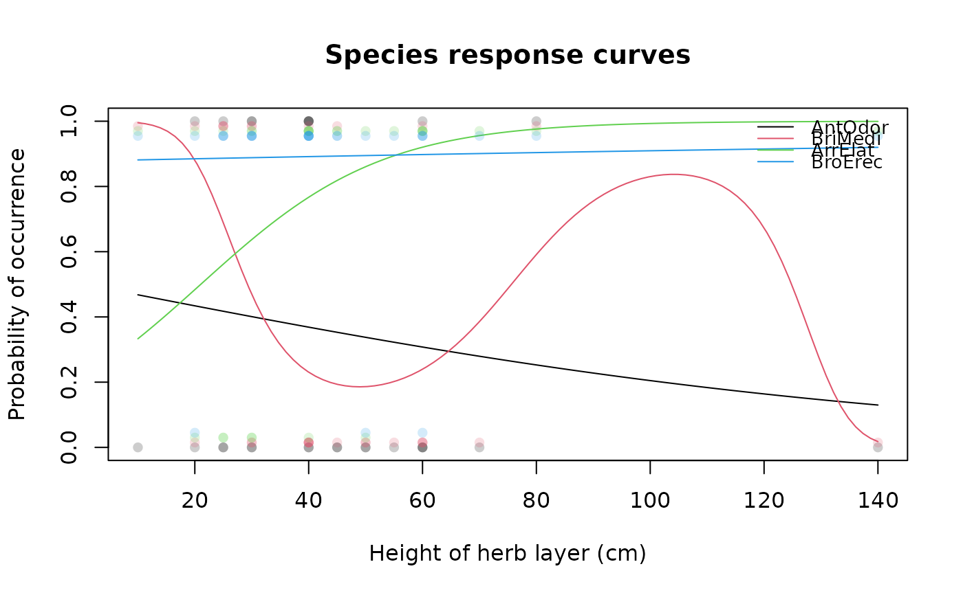
## Draw multiple species response curves on variable with
## custom x-axis label and points of occurrences
specresponse(schedenveg[ ,c(9,18,14,19)], schedenenv$height_herb,
xlab = "Height of herb layer (cm)", points = TRUE)
#> [1] "GAM with 3 knots fitted for AntOdor. Deviance explained: 1.6%, p-value = 0.478."
#> [1] "GAM with 6 knots fitted for BriMedi. Deviance explained: 20.4%, p-value = 0.191."
#> [1] "GAM with 5 knots fitted for ArrElat. Deviance explained: 16.8%, p-value = 0.187."
#> [1] "GAM with 5 knots fitted for BroErec. Deviance explained: 0.1%, p-value = 0.9."
## Draw multiple species response curves on variable with
## custom x-axis label and points of occurrences
specresponse(schedenveg[ ,c(9,18,14,19)], schedenenv$height_herb,
xlab = "Height of herb layer (cm)", points = TRUE)
 #> [1] "GLM with 1 degrees fitted for AntOdor. Deviance explained: 1.6%, p-value = 0.447."
#> [1] "GLM with 3 degrees fitted for BriMedi. Deviance explained: 21.6%, p-value = 0.044."
#> [1] "GLM with 1 degrees fitted for ArrElat. Deviance explained: 14.5%, p-value = 0.033."
#> [1] "GLM with 1 degrees fitted for BroErec. Deviance explained: 0.1%, p-value = 0.898."
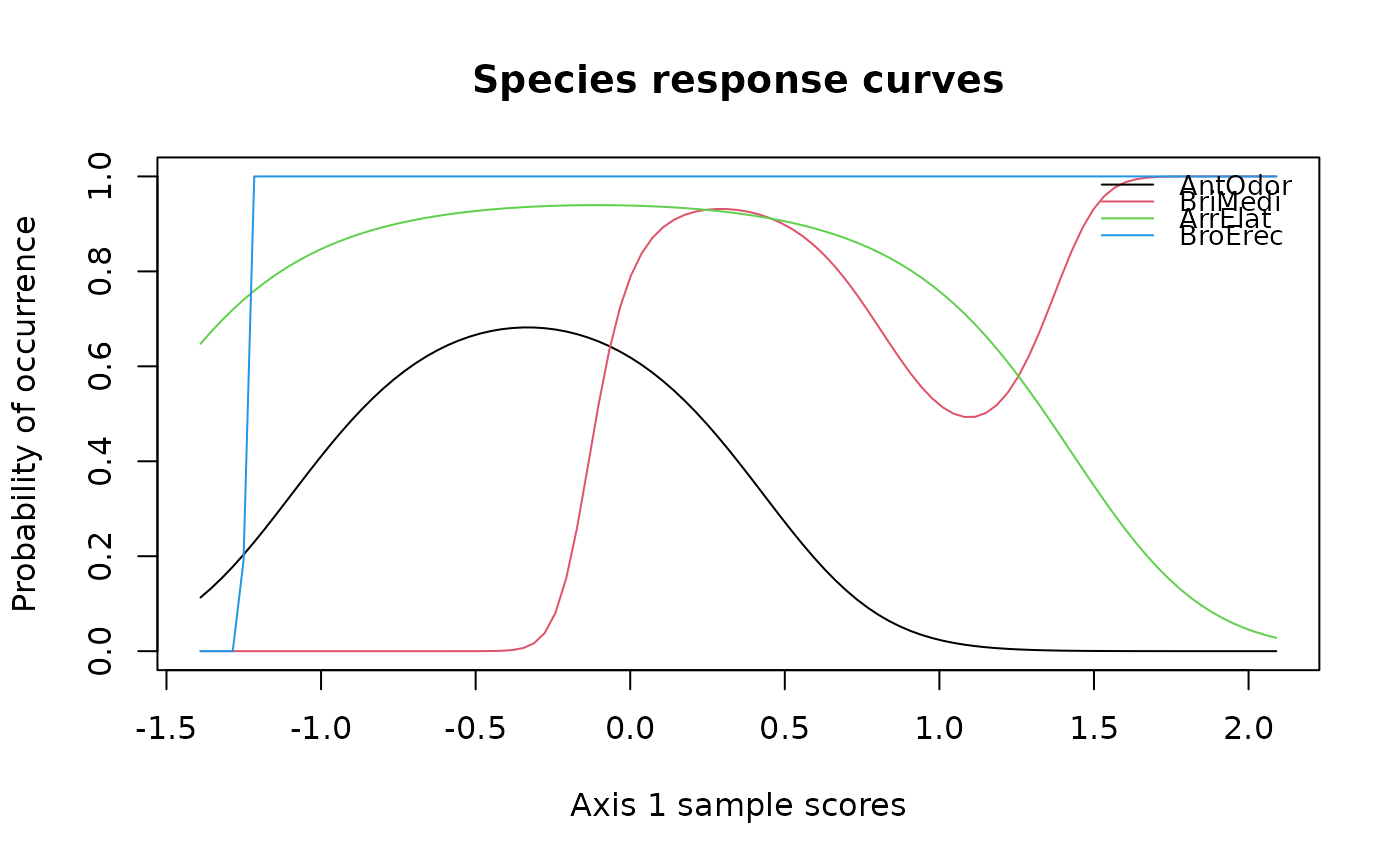
## Draw multiple species response curves on ordination axes
specresponse(schedenveg[ ,c(9,18,14,19)], scheden.dca, method = "ord")
#> [1] "GLM with 1 degrees fitted for AntOdor. Deviance explained: 1.6%, p-value = 0.447."
#> [1] "GLM with 3 degrees fitted for BriMedi. Deviance explained: 21.6%, p-value = 0.044."
#> [1] "GLM with 1 degrees fitted for ArrElat. Deviance explained: 14.5%, p-value = 0.033."
#> [1] "GLM with 1 degrees fitted for BroErec. Deviance explained: 0.1%, p-value = 0.898."
## Draw multiple species response curves on ordination axes
specresponse(schedenveg[ ,c(9,18,14,19)], scheden.dca, method = "ord")
 #> [1] "GLM with 2 degrees fitted for AntOdor. Deviance explained: 26.9%, p-value = 0.007."
#> [1] "GLM with 3 degrees fitted for BriMedi. Deviance explained: 69.2%, p-value < 0.001."
#> [1] "GLM with 2 degrees fitted for ArrElat. Deviance explained: 31%, p-value = 0.008."
#> [1] "GLM with 1 degrees fitted for BroErec. Deviance explained: 100%, p-value < 0.001."
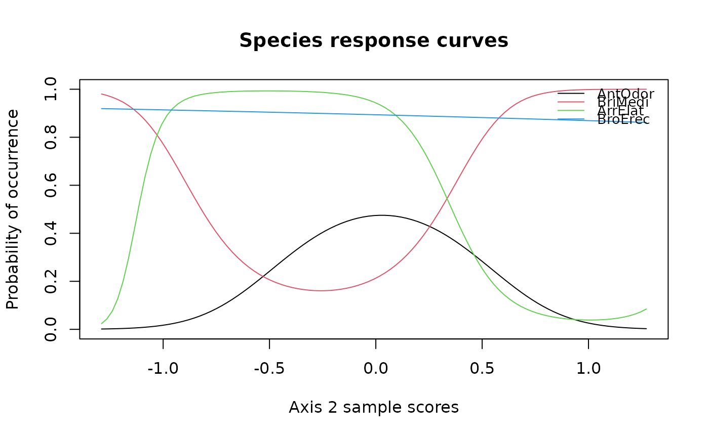
specresponse(schedenveg[ ,c(9,18,14,19)], scheden.dca, method = "ord", axis = 2)
#> [1] "GLM with 2 degrees fitted for AntOdor. Deviance explained: 26.9%, p-value = 0.007."
#> [1] "GLM with 3 degrees fitted for BriMedi. Deviance explained: 69.2%, p-value < 0.001."
#> [1] "GLM with 2 degrees fitted for ArrElat. Deviance explained: 31%, p-value = 0.008."
#> [1] "GLM with 1 degrees fitted for BroErec. Deviance explained: 100%, p-value < 0.001."
specresponse(schedenveg[ ,c(9,18,14,19)], scheden.dca, method = "ord", axis = 2)
 #> [1] "GLM with 2 degrees fitted for AntOdor. Deviance explained: 8.4%, p-value = 0.216."
#> [1] "GLM with 2 degrees fitted for BriMedi. Deviance explained: 19.5%, p-value = 0.026."
#> [1] "GLM with 3 degrees fitted for ArrElat. Deviance explained: 38.9%, p-value = 0.007."
#> [1] "GLM with 1 degrees fitted for BroErec. Deviance explained: 0.2%, p-value = 0.858."
#> [1] "GLM with 2 degrees fitted for AntOdor. Deviance explained: 8.4%, p-value = 0.216."
#> [1] "GLM with 2 degrees fitted for BriMedi. Deviance explained: 19.5%, p-value = 0.026."
#> [1] "GLM with 3 degrees fitted for ArrElat. Deviance explained: 38.9%, p-value = 0.007."
#> [1] "GLM with 1 degrees fitted for BroErec. Deviance explained: 0.2%, p-value = 0.858."