Add layers to a lattice plot, optionally using a new data source
layer.RdA mechanism to add new layers to a trellis object, optionally using a
new data source. This is an alternative to modifying the
panel function. Note the non-standard evaluation in layer().
layer(..., data, magicdots, exclude,
      packets, rows, columns, groups,
      style, force, theme, under, superpose)

layer_(...)
glayer(...)
glayer_(...)

# S3 method for class 'trellis'
object + lay

drawLayer(lay, panelArgs = trellis.panelArgs())

flattenPanel(object)
Arguments
- ...
expressions as they would appear in a panel function. These can refer to the panel function arguments (such as
x,yandsubscripts), and also to any named objects passed in through thedataargument. The calls can also include the special argument “...”; in the default case ofmagicdots = TRUE, only those arguments which are not already named in a call are passed on through “...”. Otherwise, “...” simply represents all panel function arguments. See Details, below.- data
optional. A named
listcontaining objects needed when evaluating (drawing) the layer.- magicdots, exclude
if
magicdots = TRUE, the default, any reference to “...” in the layer expressions will only pass on those arguments from the panel function which are not named in the call (thus avoiding duplicate argument errors). If the first argument in a call is not named, it is assumed to be named"x", and if the second argument is not named it is assumed to be named"y". Furthermore, any argument names given inexcludewill not be passed on through “...”.- packets, rows, columns, groups
restricts the layer to draw only in specified packets (which refer to individual panels, but are independent of their layout), or rows or columns of the trellis layout (
trellis.currentLayout). For group layers (usingglayerorsuperpose = TRUE), the groups can be restricted also, by specifying group numbers (or group values, as character strings). Negative values exclude the given items.- style
style index of the layer, used only to set lattice graphical parameters (same effect as in grouped displays). Note that this will use the theme settings in effect in the existing plot, which may or may not be what is desired. It may be necessary to use
force =
      TRUE
to escape from the plot's settings and use the current theme.- force
force = TRUEis just a shorthand fortheme = trellis.par.get(), which is useful for over-riding the theme settings in effect in an existing plot. For instance, if the original plot specifiedpar.settings = simpleTheme(col = "red")then the theme settings in effect will be entirely red. Useforce = TRUEto reset the current theme for this layer, or usethemedirectly.- theme
a style specification to be passed to
trellis.par.setwhich has effect only while drawing the layer. One can pass a whole theme specification list, such astheme = custom.theme(), or a more specific list, such astheme = simpleTheme(col = "red").- under
whether the layer should be drawn before the existing panel function. This defaults to
TRUEin the convenience functionslayer_()andglayer_().- superpose
if
TRUE, the layer will be drawn once for each level of anygroupsin the plot, usingpanel.superpose. This defaults toTRUEin the convenience functionsglayer()andglayer_().- object
a trellis object.
- lay
a layer object.
- panelArgs
list of arguments to the panel function.
Details
The layer mechanism is a method for augmenting a panel
function. It allows expressions to be added to the panel function
without knowing what the original panel function was. In this way it
can be useful for convenient augmentation of trellis plots.
Note that the evaluation used in layer is non-standard, and can
be confusing at first: you typically refer to variables as if inside
the panel function (x, y, etc); you can usually refer to
objects which exist in the global environment (workspace), but it is
safer to pass them in by name in the data argument to
layer. (And this should not to be confused with the data
argument to the original xyplot.)
A simple example is adding a reference line to each panel:
layer(panel.refline(h = 0)). Note that the expressions are
quoted, so if you have local variables they will need to be either
accessible globally, or passed in via the data argument. For
example:
layer(panel.refline(h = myVal)) ## if myVal is global
layer(panel.refline(h = h), data = list(h = myVal))
Another non-standard aspect is that the special argument
“...” will, by default, only pass through those
argument not already named. For example, this will over-ride the
x argument and pass on the remaining arguments:
layer(panel.xyplot(x = jitter(x), ...))
The first un-named argument is assumed to be "x", so that is the same as
layer(panel.xyplot(jitter(x), ...))
The layer mechanism should probably still be considered experimental.
drawLayer() actually draws the given layer object, applying the
panel specification, style settings and so on. It should only be
called while a panel is in focus.
The flattenPanel function will construct a human-readable
function incorporating code from all layers (and the original panel
function). Note that this does not return a usable function, as it
lacks the correct argument list and ignores any extra data sources
that layers might use. It is intended be edited manually.
Value
a layer object is defined as a list of expression objects,
each of which may have a set of attributes. The result of "adding"
a layer to a trellis object (+.trellis) is the updated trellis
object.
See also
update.trellis,
as.layer for overlaying entire plots
Examples
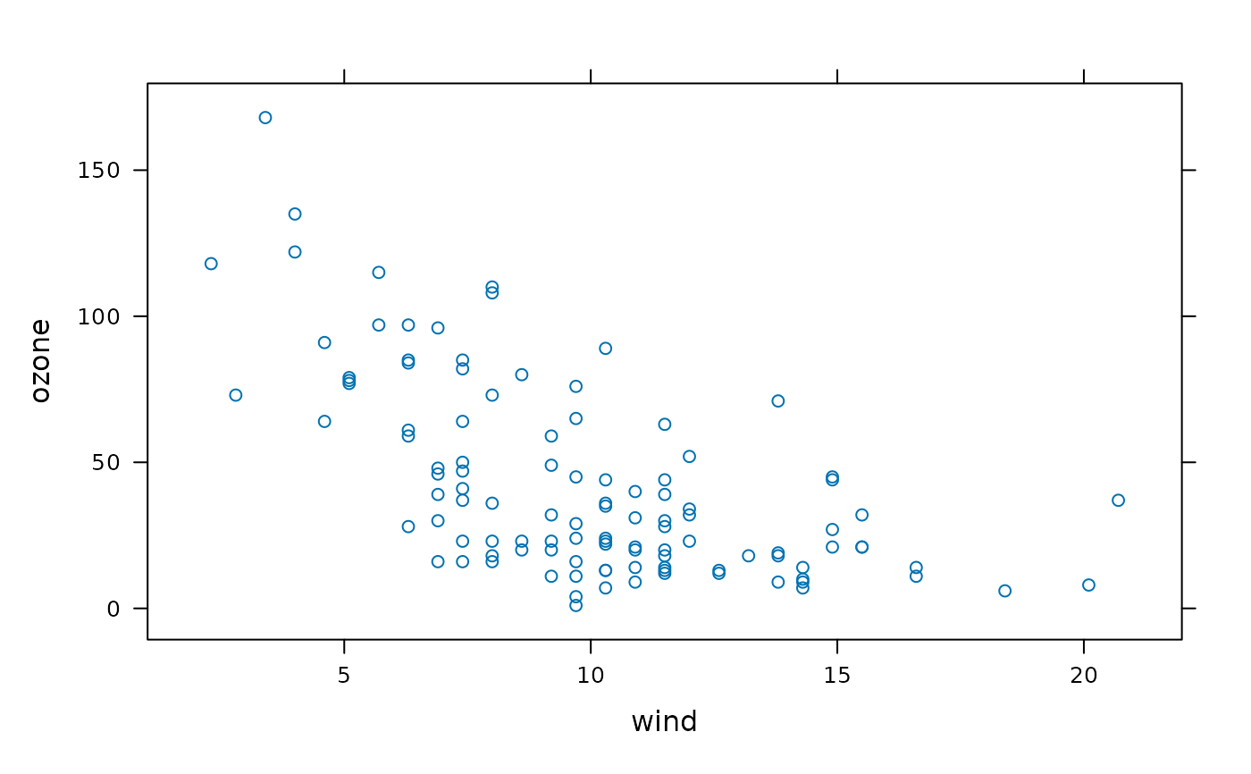
foo <- xyplot(ozone ~ wind, environmental)
foo
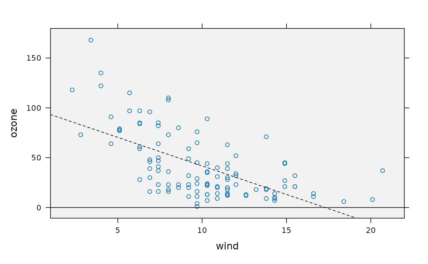
 ## overlay reference lines
foo <- foo + layer(panel.abline(h = 0)) +
layer(panel.lmline(x, y, lty = 2))
## underlay a flat color
foo <- foo + layer(panel.fill(grey(.95)), under = TRUE)
foo
## overlay reference lines
foo <- foo + layer(panel.abline(h = 0)) +
layer(panel.lmline(x, y, lty = 2))
## underlay a flat color
foo <- foo + layer(panel.fill(grey(.95)), under = TRUE)
foo
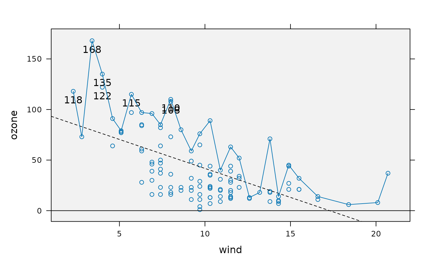
 ## layers can access the panel function arguments
foo <- foo + layer({ ok <- (y>100);
panel.text(x[ok], y[ok], y[ok], pos = 1) })
foo
## layers can access the panel function arguments
foo <- foo + layer({ ok <- (y>100);
panel.text(x[ok], y[ok], y[ok], pos = 1) })
foo
 ## over-ride arguments by name
foo <- foo +
layer(panel.xyplot(y = ave(y, x, FUN = max), type = "a", ...))
foo
## over-ride arguments by name
foo <- foo +
layer(panel.xyplot(y = ave(y, x, FUN = max), type = "a", ...))
foo
 ## see a sketch of the complete panel function
flattenPanel(foo)
#> {
#> panel.fill(grey(0.95))
#> panel.xyplot(...)
#> panel.abline(h = 0)
#> panel.lmline(x, y, lty = 2)
#> {
#> ok <- (y > 100)
#> panel.text(x[ok], y[ok], y[ok], pos = 1)
#> }
#> do.call(panel.xyplot, modifyList(list(...), list(y = ave(y,
#> x, FUN = max), type = "a")))
#> }
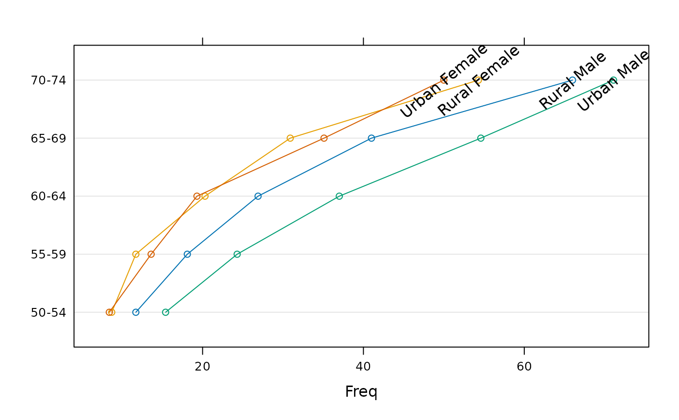
## group layers, drawn for each group in each panel
dotplot(VADeaths, type = "o") +
glayer(ltext(x[5], y[5], group.value, srt = 40))
## see a sketch of the complete panel function
flattenPanel(foo)
#> {
#> panel.fill(grey(0.95))
#> panel.xyplot(...)
#> panel.abline(h = 0)
#> panel.lmline(x, y, lty = 2)
#> {
#> ok <- (y > 100)
#> panel.text(x[ok], y[ok], y[ok], pos = 1)
#> }
#> do.call(panel.xyplot, modifyList(list(...), list(y = ave(y,
#> x, FUN = max), type = "a")))
#> }
## group layers, drawn for each group in each panel
dotplot(VADeaths, type = "o") +
glayer(ltext(x[5], y[5], group.value, srt = 40))
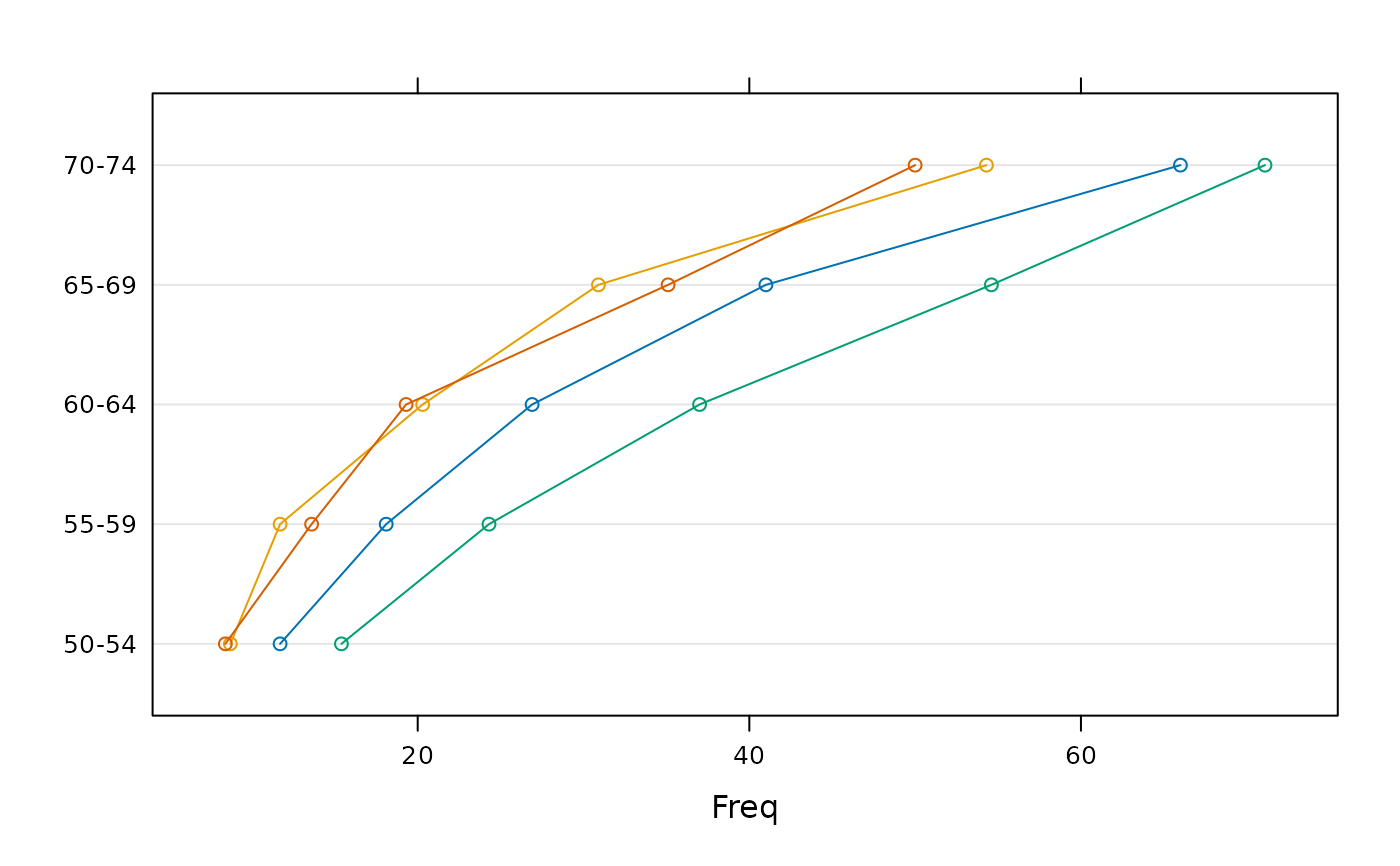
 ## a quick way to print out the panel.groups arguments:
dotplot(VADeaths, type = "o") + glayer(str(list(...)))
## a quick way to print out the panel.groups arguments:
dotplot(VADeaths, type = "o") + glayer(str(list(...)))
 #> List of 21
#> $ x : num [1:5] 11.7 18.1 26.9 41 66
#> $ subscripts : int [1:5] 1 2 3 4 5
#> $ pch : num 1
#> $ cex : num 0.8
#> $ font : num 1
#> $ fontface : NULL
#> $ fontfamily : NULL
#> $ col : chr "black"
#> $ col.line : chr "#0072B2"
#> $ col.symbol : chr "#0072B2"
#> $ fill : chr "#CCFFFF"
#> $ lty : num 1
#> $ lwd : num 1
#> $ alpha : num 1
#> $ type : chr "o"
#> $ group.number: int 1
#> $ group.value : chr "Rural Male"
#> $ grid : logi FALSE
#> $ box.ratio : num 1
#> $ horizontal : logi TRUE
#> $ y : num [1:5] 1 2 3 4 5
#> List of 21
#> $ x : num [1:5] 8.7 11.7 20.3 30.9 54.3
#> $ subscripts : int [1:5] 6 7 8 9 10
#> $ pch : num 1
#> $ cex : num 0.8
#> $ font : num 1
#> $ fontface : NULL
#> $ fontfamily : NULL
#> $ col : chr "black"
#> $ col.line : chr "#E69F00"
#> $ col.symbol : chr "#E69F00"
#> $ fill : chr "#FFCCFF"
#> $ lty : num 1
#> $ lwd : num 1
#> $ alpha : num 1
#> $ type : chr "o"
#> $ group.number: int 2
#> $ group.value : chr "Rural Female"
#> $ grid : logi FALSE
#> $ box.ratio : num 1
#> $ horizontal : logi TRUE
#> $ y : num [1:5] 1 2 3 4 5
#> List of 21
#> $ x : num [1:5] 15.4 24.3 37 54.6 71.1
#> $ subscripts : int [1:5] 11 12 13 14 15
#> $ pch : num 1
#> $ cex : num 0.8
#> $ font : num 1
#> $ fontface : NULL
#> $ fontfamily : NULL
#> $ col : chr "black"
#> $ col.line : chr "#009E73"
#> $ col.symbol : chr "#009E73"
#> $ fill : chr "#CCFFCC"
#> $ lty : num 1
#> $ lwd : num 1
#> $ alpha : num 1
#> $ type : chr "o"
#> $ group.number: int 3
#> $ group.value : chr "Urban Male"
#> $ grid : logi FALSE
#> $ box.ratio : num 1
#> $ horizontal : logi TRUE
#> $ y : num [1:5] 1 2 3 4 5
#> List of 21
#> $ x : num [1:5] 8.4 13.6 19.3 35.1 50
#> $ subscripts : int [1:5] 16 17 18 19 20
#> $ pch : num 1
#> $ cex : num 0.8
#> $ font : num 1
#> $ fontface : NULL
#> $ fontfamily : NULL
#> $ col : chr "black"
#> $ col.line : chr "#D55E00"
#> $ col.symbol : chr "#D55E00"
#> $ fill : chr "#FFE5CC"
#> $ lty : num 1
#> $ lwd : num 1
#> $ alpha : num 1
#> $ type : chr "o"
#> $ group.number: int 4
#> $ group.value : chr "Urban Female"
#> $ grid : logi FALSE
#> $ box.ratio : num 1
#> $ horizontal : logi TRUE
#> $ y : num [1:5] 1 2 3 4 5
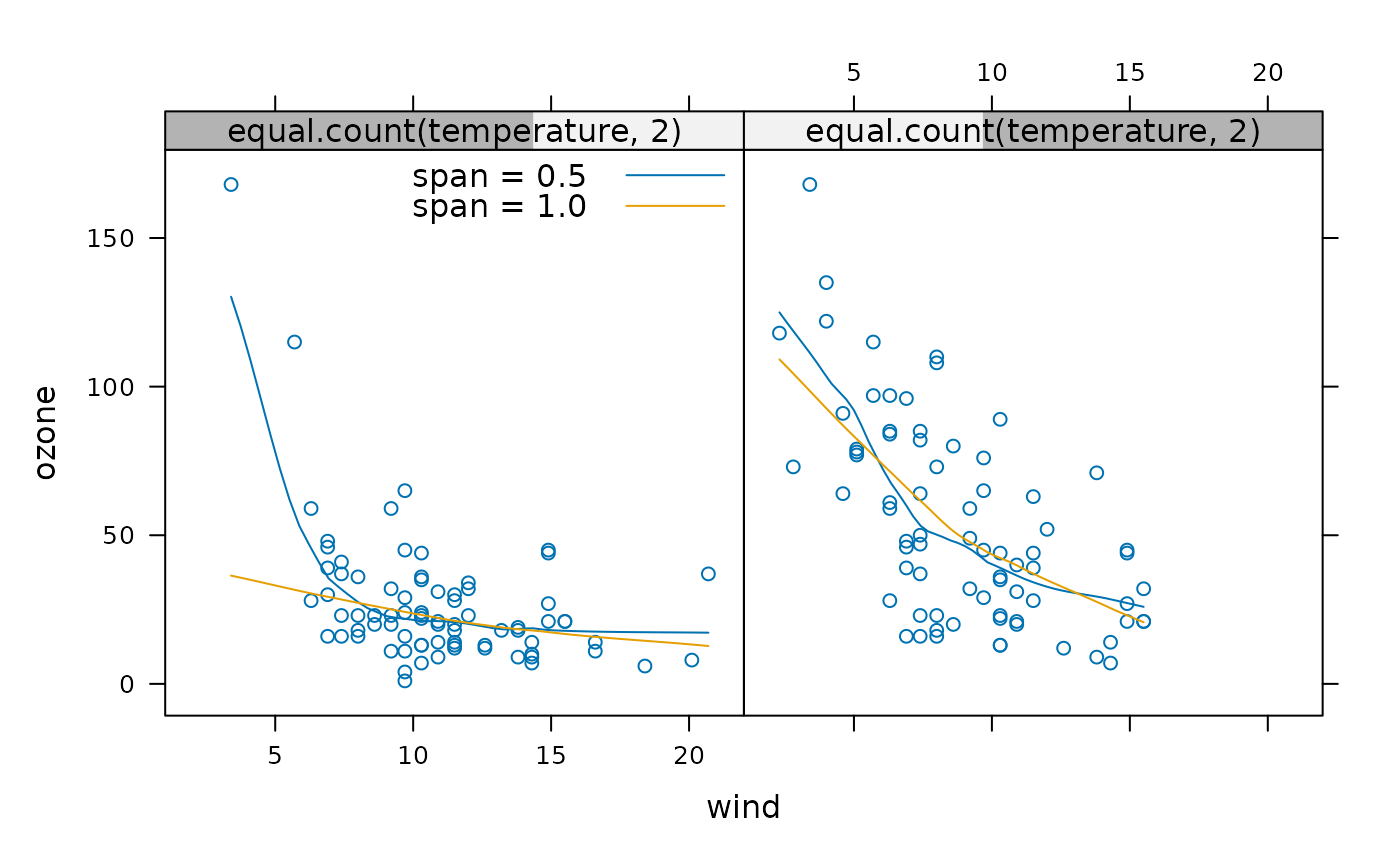
## layers with superposed styles
xyplot(ozone ~ wind | equal.count(temperature, 2),
data = environmental) +
layer(panel.loess(x, y, span = 0.5), style = 1) +
layer(panel.loess(x, y, span = 1.0), style = 2) +
layer(panel.key(c("span = 0.5", "span = 1.0"), corner = c(1,.98),
lines = TRUE, points = FALSE), packets = 1)
#> List of 21
#> $ x : num [1:5] 11.7 18.1 26.9 41 66
#> $ subscripts : int [1:5] 1 2 3 4 5
#> $ pch : num 1
#> $ cex : num 0.8
#> $ font : num 1
#> $ fontface : NULL
#> $ fontfamily : NULL
#> $ col : chr "black"
#> $ col.line : chr "#0072B2"
#> $ col.symbol : chr "#0072B2"
#> $ fill : chr "#CCFFFF"
#> $ lty : num 1
#> $ lwd : num 1
#> $ alpha : num 1
#> $ type : chr "o"
#> $ group.number: int 1
#> $ group.value : chr "Rural Male"
#> $ grid : logi FALSE
#> $ box.ratio : num 1
#> $ horizontal : logi TRUE
#> $ y : num [1:5] 1 2 3 4 5
#> List of 21
#> $ x : num [1:5] 8.7 11.7 20.3 30.9 54.3
#> $ subscripts : int [1:5] 6 7 8 9 10
#> $ pch : num 1
#> $ cex : num 0.8
#> $ font : num 1
#> $ fontface : NULL
#> $ fontfamily : NULL
#> $ col : chr "black"
#> $ col.line : chr "#E69F00"
#> $ col.symbol : chr "#E69F00"
#> $ fill : chr "#FFCCFF"
#> $ lty : num 1
#> $ lwd : num 1
#> $ alpha : num 1
#> $ type : chr "o"
#> $ group.number: int 2
#> $ group.value : chr "Rural Female"
#> $ grid : logi FALSE
#> $ box.ratio : num 1
#> $ horizontal : logi TRUE
#> $ y : num [1:5] 1 2 3 4 5
#> List of 21
#> $ x : num [1:5] 15.4 24.3 37 54.6 71.1
#> $ subscripts : int [1:5] 11 12 13 14 15
#> $ pch : num 1
#> $ cex : num 0.8
#> $ font : num 1
#> $ fontface : NULL
#> $ fontfamily : NULL
#> $ col : chr "black"
#> $ col.line : chr "#009E73"
#> $ col.symbol : chr "#009E73"
#> $ fill : chr "#CCFFCC"
#> $ lty : num 1
#> $ lwd : num 1
#> $ alpha : num 1
#> $ type : chr "o"
#> $ group.number: int 3
#> $ group.value : chr "Urban Male"
#> $ grid : logi FALSE
#> $ box.ratio : num 1
#> $ horizontal : logi TRUE
#> $ y : num [1:5] 1 2 3 4 5
#> List of 21
#> $ x : num [1:5] 8.4 13.6 19.3 35.1 50
#> $ subscripts : int [1:5] 16 17 18 19 20
#> $ pch : num 1
#> $ cex : num 0.8
#> $ font : num 1
#> $ fontface : NULL
#> $ fontfamily : NULL
#> $ col : chr "black"
#> $ col.line : chr "#D55E00"
#> $ col.symbol : chr "#D55E00"
#> $ fill : chr "#FFE5CC"
#> $ lty : num 1
#> $ lwd : num 1
#> $ alpha : num 1
#> $ type : chr "o"
#> $ group.number: int 4
#> $ group.value : chr "Urban Female"
#> $ grid : logi FALSE
#> $ box.ratio : num 1
#> $ horizontal : logi TRUE
#> $ y : num [1:5] 1 2 3 4 5
## layers with superposed styles
xyplot(ozone ~ wind | equal.count(temperature, 2),
data = environmental) +
layer(panel.loess(x, y, span = 0.5), style = 1) +
layer(panel.loess(x, y, span = 1.0), style = 2) +
layer(panel.key(c("span = 0.5", "span = 1.0"), corner = c(1,.98),
lines = TRUE, points = FALSE), packets = 1)
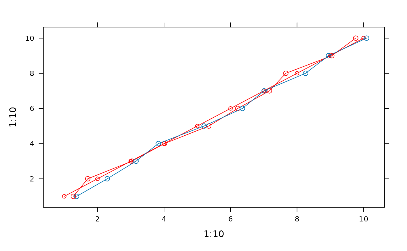
 ## note that styles come from the settings in effect in the plot,
## which is not always what you want:
xyplot(1:10 ~ 1:10, type = "b", par.settings = simpleTheme(col = "red")) +
layer(panel.lines(x = jitter(x, 2), ...)) + ## drawn in red
layer(panel.lines(x = jitter(x, 2), ...), force = TRUE) ## reset theme
## note that styles come from the settings in effect in the plot,
## which is not always what you want:
xyplot(1:10 ~ 1:10, type = "b", par.settings = simpleTheme(col = "red")) +
layer(panel.lines(x = jitter(x, 2), ...)) + ## drawn in red
layer(panel.lines(x = jitter(x, 2), ...), force = TRUE) ## reset theme
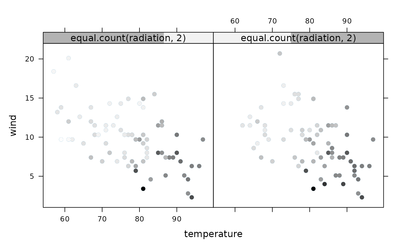
 ## using other variables from the original `data` object
## NOTE: need subscripts = TRUE in original call!
zoip <- xyplot(wind ~ temperature | equal.count(radiation, 2),
data = environmental, subscripts = TRUE)
zoip + layer(panel.points(..., pch = 19,
col = grey(1 - ozone[subscripts] / max(ozone))),
data = environmental)
## using other variables from the original `data` object
## NOTE: need subscripts = TRUE in original call!
zoip <- xyplot(wind ~ temperature | equal.count(radiation, 2),
data = environmental, subscripts = TRUE)
zoip + layer(panel.points(..., pch = 19,
col = grey(1 - ozone[subscripts] / max(ozone))),
data = environmental)
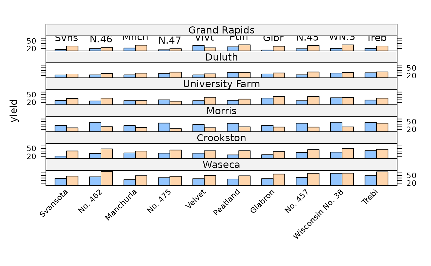
 ## restrict drawing to specified panels
barchart(yield ~ variety | site, data = barley,
groups = year, layout = c(1,6), as.table = TRUE,
scales = list(x = list(rot = 45))) +
layer(ltext(tapply(y, x, max), lab = abbreviate(levels(x)),
pos = 3), rows = 1)
## restrict drawing to specified panels
barchart(yield ~ variety | site, data = barley,
groups = year, layout = c(1,6), as.table = TRUE,
scales = list(x = list(rot = 45))) +
layer(ltext(tapply(y, x, max), lab = abbreviate(levels(x)),
pos = 3), rows = 1)
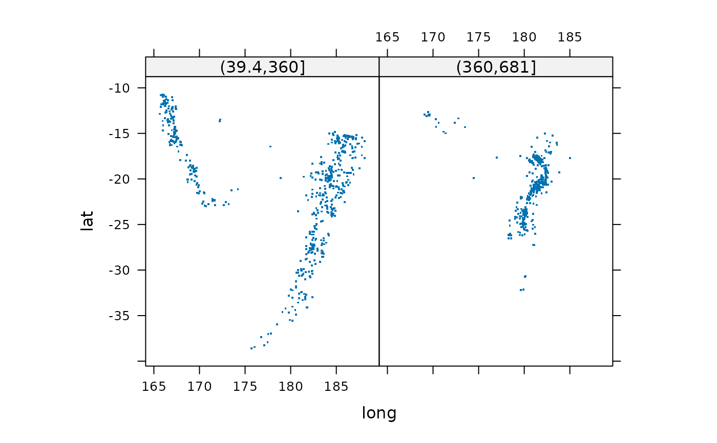
 ## example of a new data source
qua <- xyplot(lat ~ long | cut(depth, 2), quakes,
aspect = "iso", pch = ".", cex = 2)
qua
## example of a new data source
qua <- xyplot(lat ~ long | cut(depth, 2), quakes,
aspect = "iso", pch = ".", cex = 2)
qua
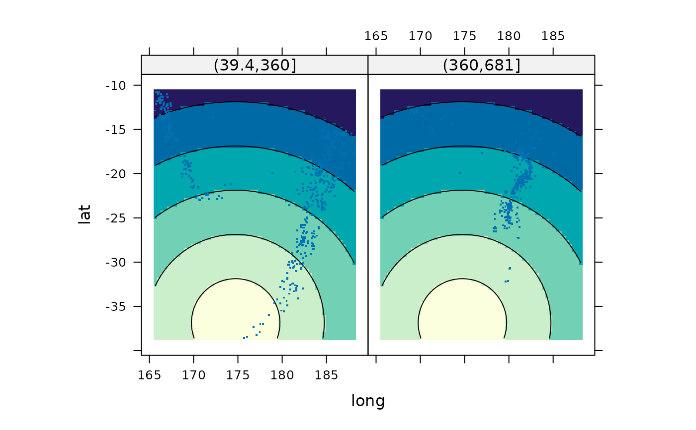
 ## add layer showing distance from Auckland
newdat <- with(quakes, expand.grid(
gridlat = seq(min(lat), max(lat), length = 60),
gridlon = seq(min(long), max(long), length = 60)))
newdat$dist <- with(newdat, sqrt((gridlat - -36.87)^2 +
(gridlon - 174.75)^2))
qua + layer_(panel.contourplot(x = gridlon, y = gridlat, z = dist,
contour = TRUE, subscripts = TRUE), data = newdat)
## add layer showing distance from Auckland
newdat <- with(quakes, expand.grid(
gridlat = seq(min(lat), max(lat), length = 60),
gridlon = seq(min(long), max(long), length = 60)))
newdat$dist <- with(newdat, sqrt((gridlat - -36.87)^2 +
(gridlon - 174.75)^2))
qua + layer_(panel.contourplot(x = gridlon, y = gridlat, z = dist,
contour = TRUE, subscripts = TRUE), data = newdat)