Trellis Displays of Tukey's Hanging Rootograms

Displays hanging rootograms.

rootogram(x, ...)

# S3 method for class 'formula'
rootogram(x, data = parent.frame(),
          ylab = expression(sqrt(P(X == x))),
          prepanel = prepanel.rootogram,
          panel = panel.rootogram,
          ...,
          probability = TRUE)

prepanel.rootogram(x, y = table(x),
                   dfun = NULL,
                   transformation = sqrt,
                   hang = TRUE,
                   probability = TRUE,
                   ...)

panel.rootogram(x, y = table(x),
                dfun = NULL,
                col = plot.line$col,
                lty = plot.line$lty,
                lwd = plot.line$lwd,
                alpha = plot.line$alpha,
                transformation = sqrt,
                hang = TRUE,
                probability = TRUE,
                type = "l", pch = 16,
                ...)

Arguments

x, y

For rootogram, x is the object on which method dispatch is carried out. For the "formula" method, x is a formula describing the form of conditioning plot. The formula can be either of the form ~x or of the form y~x. In the first case, x is assumed to be a vector of raw observations, and an observed frequency distribution is computed from it. In the second case, x is assumed to be unique values and y the corresponding frequencies. In either case, further conditioning variables are allowed.

A similar interpretation holds for x and y in prepanel.rootogram and panel.rootogram.

Note that the data are assumed to arise from a discrete distribution with some probability mass function. See details below.

data

For the "formula" method, a data frame containing values for any variables in the formula, as well as those in groups and subset if applicable (groups is currently ignored by the default panel function). By default the environment where the function was called from is used.

dfun

a probability mass function, to be evaluated at unique x values

prepanel, panel

panel and prepanel function used to create the display.

ylab

the y-axis label; typically a character string or an expression.

col, lty, lwd, alpha

graphical parameters

transformation

a vectorized function. Relative frequencies (observed) and theoretical probabilities (dfun) are transformed by this function before being plotted.

hang

logical, whether lines representing observed relative freuqncies should “hang” from the curve representing the theoretical probabilities.

probability

A logical flag, controlling whether the y-values are to be standardized to be probabilities by dividing by their sum.

type

A character vector consisting of one or both of "p" and "l". If "p" is included, the evaluated values of dfun will be denoted by points, and if "l" is included, they will be joined by lines.

pch

The plotting character to be used for the "p" type.

...

extra arguments, passed on as appropriate. Standard lattice arguments as well as arguments to panel.rootogram can be supplied directly in the high level rootogram call.

Details

This function implements Tukey's hanging rootograms. As implemented, rootogram assumes that the data arise from a discrete distribution (either supplied in raw form, when y is unspecified, or in terms of the frequency distribution) with some unknown probability mass function (p.m.f.). The purpose of the plot is to check whether the supplied theoretical p.m.f. dfun is a reasonable fit for the data.

It is reasonable to consider rootograms for continuous data by discretizing it (similar to a histogram), but this must be done by the user before calling rootogram. An example is given below.

Also consider the rootogram function in the vcd package, especially if the number of unique values is small.

Value

rootogram produces an object of class "trellis". The update method can be used to update components of the object and the print method (usually called by default) will plot it on an appropriate plotting device.

References

John W. Tukey (1972) Some graphic and semi-graphic displays. In T. A. Bancroft (Ed) Statistical Papers in Honor of George W. Snedecor, pp. 293–316. Available online at https://www.edwardtufte.com/tufte/tukey

Author

Deepayan Sarkar deepayan.sarkar@gmail.com

Examples


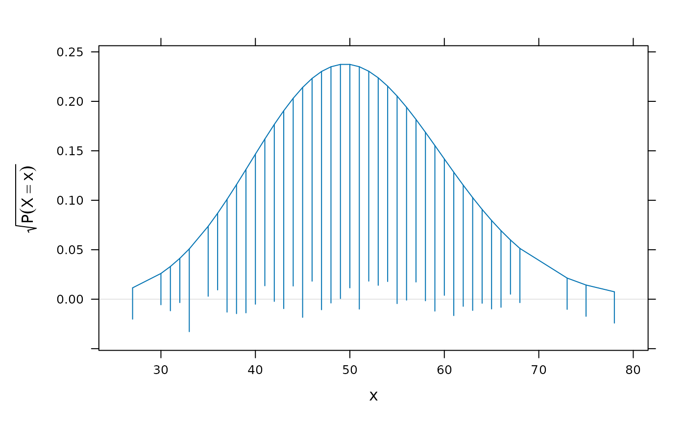
library(lattice)

x <- rpois(1000, lambda = 50)

p <- rootogram(~x, dfun = function(x) dpois(x, lambda = 50))
p


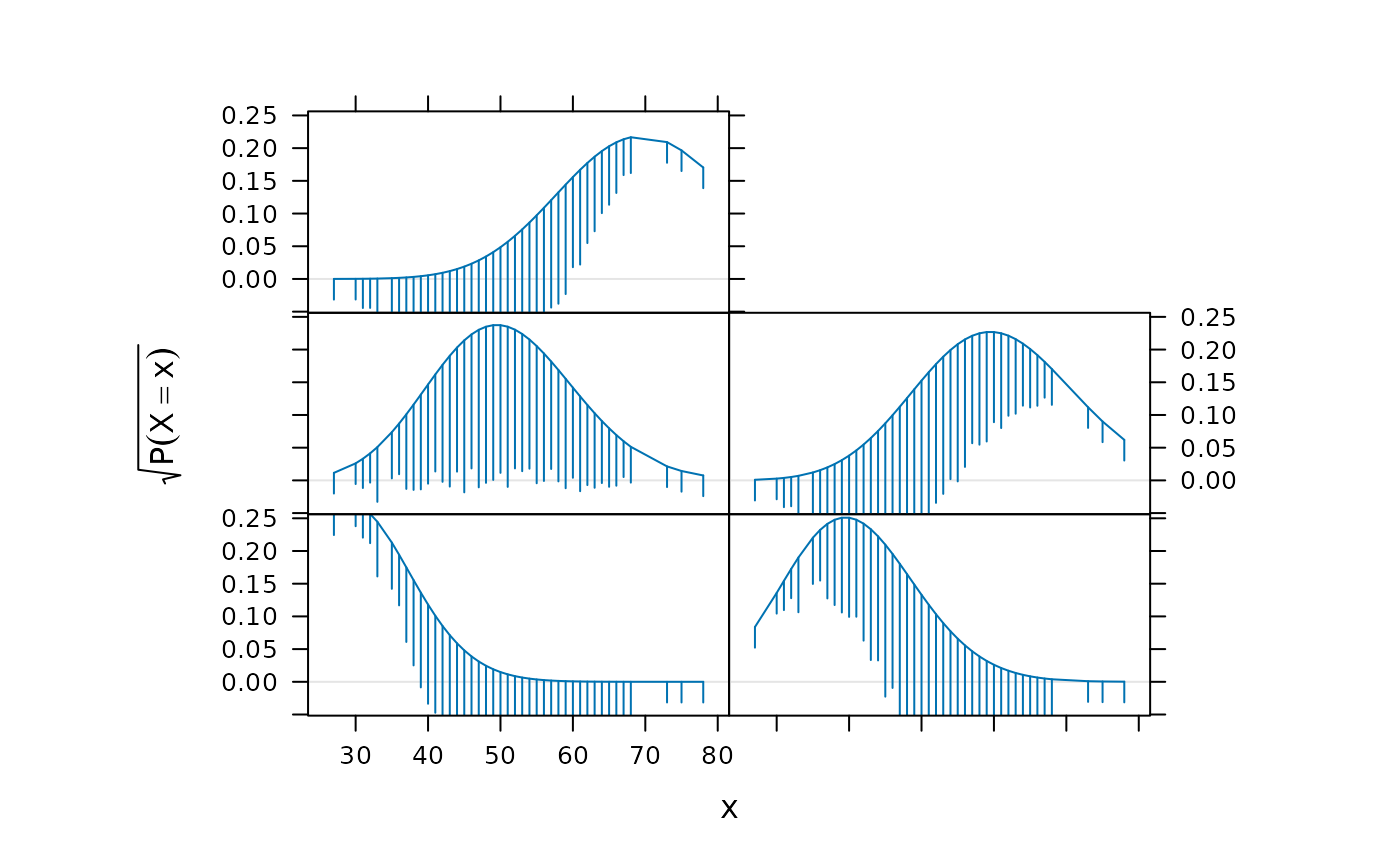
lambdav <- c(30, 40, 50, 60, 70)

update(p[rep(1, length(lambdav))],
       aspect = "xy",
       panel = function(x, ...) {
           panel.rootogram(x,
                           dfun = function(x)
                           dpois(x, lambda = lambdav[panel.number()]))
       })



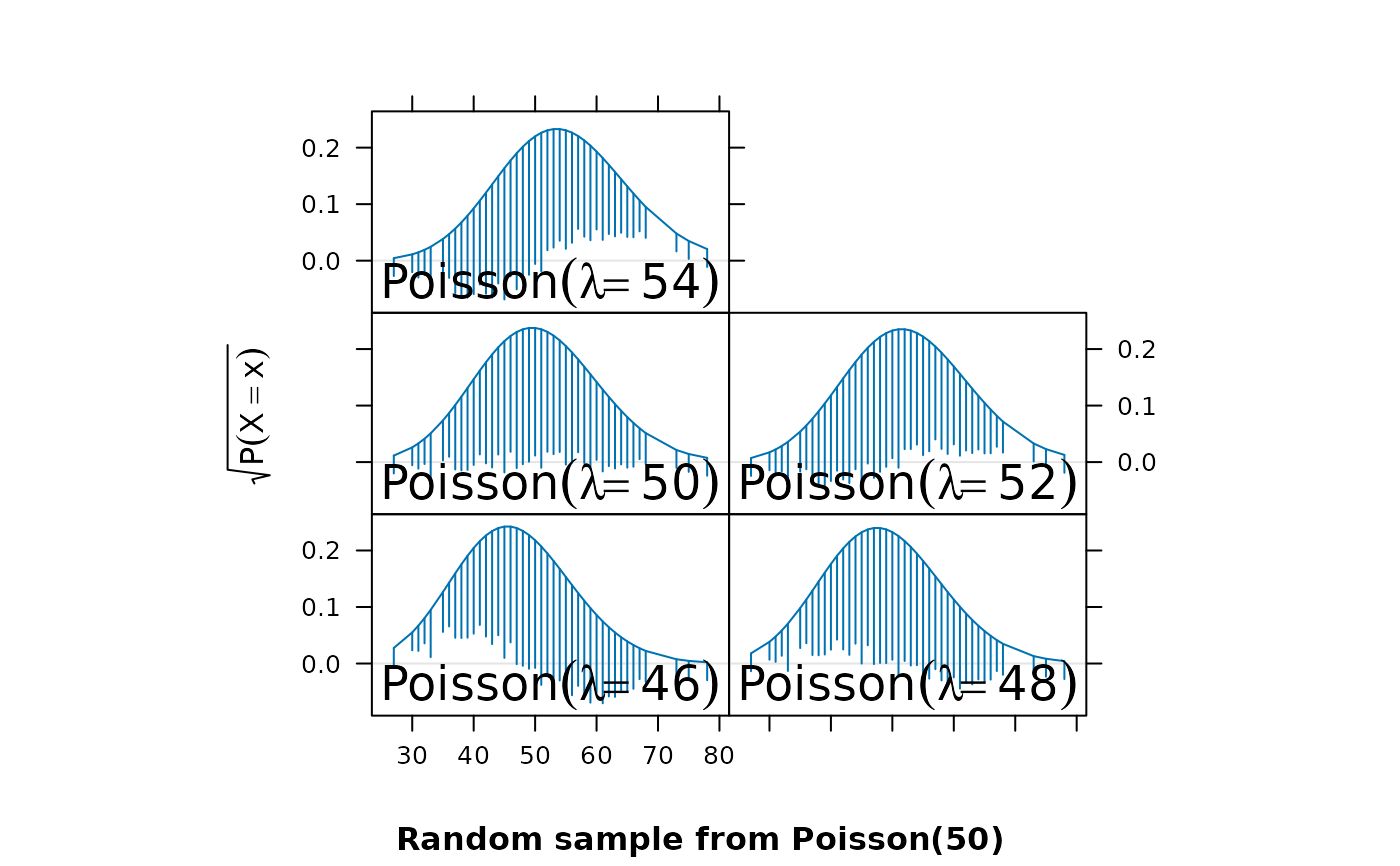
lambdav <- c(46, 48, 50, 52, 54)

update(p[rep(1, length(lambdav))],
       aspect = "xy",
       prepanel = function(x, ...) {
           tmp <-
               lapply(lambdav,
                      function(lambda) {
                          prepanel.rootogram(x,
                                             dfun = function(x)
                                             dpois(x, lambda = lambda))
                      })
           list(xlim = range(sapply(tmp, "[[", "xlim")),
                ylim = range(sapply(tmp, "[[", "ylim")),
                dx = do.call("c", lapply(tmp, "[[", "dx")),
                dy = do.call("c", lapply(tmp, "[[", "dy")))
       },
       panel = function(x, ...) {
           panel.rootogram(x,
                           dfun = function(x)
                           dpois(x, lambda = lambdav[panel.number()]))
           grid::grid.text(bquote(Poisson(lambda == .(foo)),
                                  where = list(foo = lambdav[panel.number()])),
                           y = 0.15,
                           gp = grid::gpar(cex = 1.5))
       },
       xlab = "",
       sub = "Random sample from Poisson(50)")



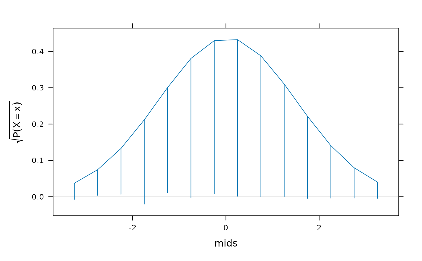
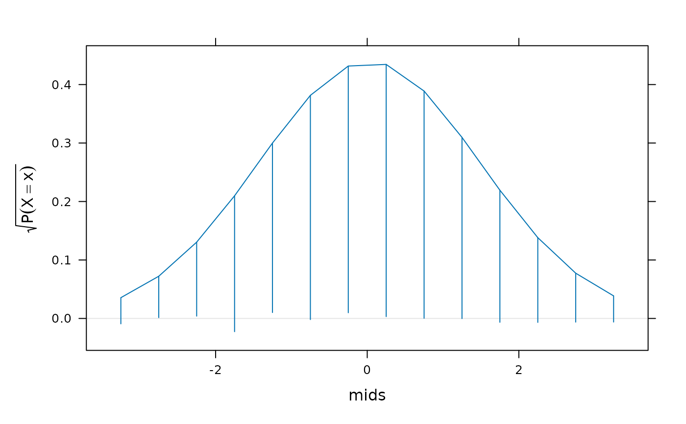
## Example using continuous data

xnorm <- rnorm(1000)

## 'discretize' by binning and replacing data by bin midpoints

h <- hist(xnorm, plot = FALSE)

## Option 1: Assume bin probabilities proportional to dnorm()

norm.factor <- sum(dnorm(h$mids, mean(xnorm), sd(xnorm)))

rootogram(counts ~ mids, data = h,
          dfun = function(x) {
              dnorm(x, mean(xnorm), sd(xnorm)) / norm.factor
          })


## Option 2: Compute probabilities explicitly using pnorm()

pdisc <- diff(pnorm(h$breaks, mean = mean(xnorm), sd = sd(xnorm)))
pdisc <- pdisc / sum(pdisc)

rootogram(counts ~ mids, data = h,
          dfun = function(x) {
              f <- factor(x, levels = h$mids)
              pdisc[f]
          })