Regression model for binomial data with unkown group of immortals (zero-inflated binomial regression)
zibreg(
  formula,
  formula.p = ~1,
  data,
  family = stats::binomial(),
  offset = NULL,
  start,
  var = "hessian",
  ...
)
Arguments
- formula
Formula specifying
- formula.p
Formula for model of disease prevalence
- data
data frame
- family
Distribution family (see the help page
family)- offset
Optional offset
- start
Optional starting values
- var
Type of variance (robust, expected, hessian, outer)
- ...
Additional arguments to lower level functions
Examples
## Simulation
n <- 2e3
x <- runif(n,0,20)
age <- runif(n,10,30)
z0 <- rnorm(n,mean=-1+0.05*age)
z <- cut(z0,breaks=c(-Inf,-1,0,1,Inf))
p0 <- lava:::expit(model.matrix(~z+age) %*% c(-.4, -.4, 0.2, 2, -0.05))
y <- (runif(n)<lava:::tigol(-1+0.25*x-0*age))*1
u <- runif(n)<p0
y[u==0] <- 0
d <- data.frame(y=y,x=x,u=u*1,z=z,age=age)
head(d)
#> y x u z age
#> 1 1 3.400949 1 (-Inf,-1] 10.29035
#> 2 0 11.764343 0 (-1,0] 21.59965
#> 3 0 6.814083 0 (0,1] 26.49870
#> 4 1 15.448978 1 (1, Inf] 27.59251
#> 5 0 19.809105 0 (-1,0] 22.76442
#> 6 0 6.067391 0 (-1,0] 20.73910
## Estimation
e0 <- zibreg(y~x*z,~1+z+age,data=d)
e <- zibreg(y~x,~1+z+age,data=d)
compare(e,e0)
#>
#> - Likelihood ratio test -
#>
#> data:
#> chisq = 7.1372, df = 6, p-value = 0.3083
#> sample estimates:
#> log likelihood (model 1) log likelihood (model 2)
#> -861.9251 -858.3565
#>
e
#> Estimate 2.5% 97.5% P-value
#> (Intercept) -1.01890790 -1.65613685 -0.38167895 1.724895e-03
#> x 0.33038862 0.12632148 0.53445575 1.507586e-03
#> pr:(Intercept) -0.47967496 -1.01040085 0.05105093 7.648863e-02
#> pr:z(-1,0] -0.29790559 -0.70088729 0.10507611 1.473627e-01
#> pr:z(0,1] 0.23269232 -0.16078016 0.62616480 2.464210e-01
#> pr:z(1, Inf] 1.95961251 1.49960070 2.41962432 6.867718e-17
#> pr:age -0.05470745 -0.07869567 -0.03071923 7.826079e-06
#>
#> Prevalence probabilities:
#> Estimate 2.5% 97.5%
#> {(Intercept)} 0.3823289 0.2669014 0.5127600
#> {(Intercept)} + {z(-1,0]} 0.3148416 0.2111198 0.4410327
#> {(Intercept)} + {z(0,1]} 0.4385663 0.3071482 0.5792074
#> {(Intercept)} + {z(1, Inf]} 0.8145631 0.6882539 0.8973302
#> {(Intercept)} + {age} 0.3694953 0.2597995 0.4945617
PD(e0,intercept=c(1,3),slope=c(2,6))
#> Estimate Std.Err 2.5% 97.5%
#> 50% -0.4711308 3.002976 -6.356855 5.414594
#> attr(,"b")
#> [1] 0.2700798 0.5732587
B <- rbind(c(1,0,0,0,20),
c(1,1,0,0,20),
c(1,0,1,0,20),
c(1,0,0,1,20))
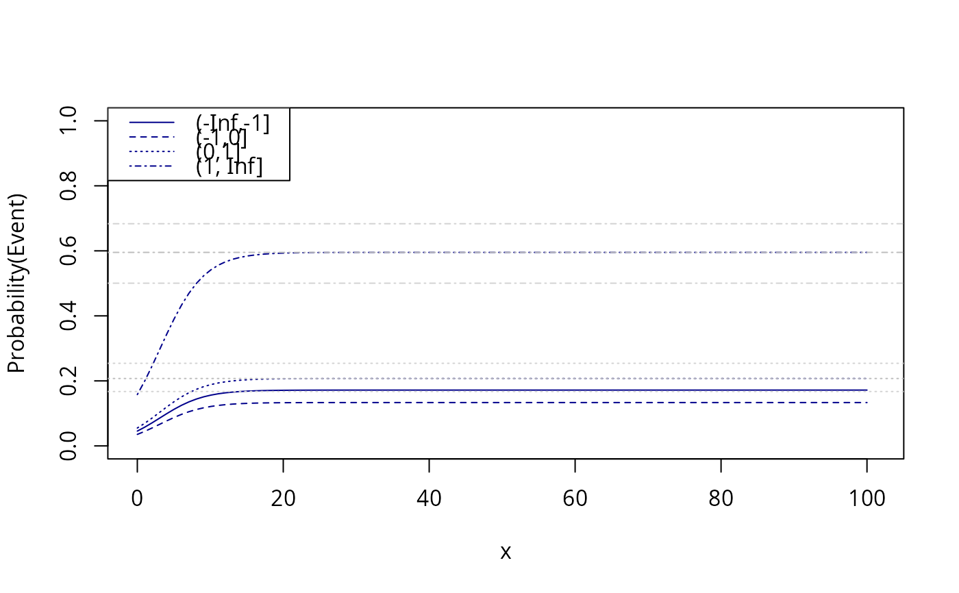
prev <- summary(e,pr.contrast=B)$prevalence
x <- seq(0,100,length.out=100)
newdata <- expand.grid(x=x,age=20,z=levels(d$z))
fit <- predict(e,newdata=newdata)
plot(0,0,type="n",xlim=c(0,101),ylim=c(0,1),xlab="x",ylab="Probability(Event)")
count <- 0
for (i in levels(newdata$z)) {
count <- count+1
lines(x,fit[which(newdata$z==i)],col="darkblue",lty=count)
}
abline(h=prev[3:4,1],lty=3:4,col="gray")
abline(h=prev[3:4,2],lty=3:4,col="lightgray")
abline(h=prev[3:4,3],lty=3:4,col="lightgray")
legend("topleft",levels(d$z),col="darkblue",lty=seq_len(length(levels(d$z))))