Verbal Aggression item responses

These are the item responses to a questionaire on verbal aggression. These data are used throughout De Boeck and Wilson (2004) to illustrate various forms of item response models.

Format

A data frame with 7584 observations on the following 13 variables.

Anger

the subject's Trait Anger score as measured on the State-Trait Anger Expression Inventory (STAXI)

Gender

the subject's gender - a factor with levels M and F

item

the item on the questionaire, as a factor

resp

the subject's response to the item - an ordered factor with levels no < perhaps < yes

id

the subject identifier, as a factor

btype

behavior type - a factor with levels curse, scold and shout

situ

situation type - a factor with levels other and self indicating other-to-blame and self-to-blame

mode

behavior mode - a factor with levels want and do

r2

dichotomous version of the response - a factor with levels N and Y

Source

Data originally from the UC Berkeley BEAR Center; original link is available at https://web.archive.org/web/20221128003829/https://old.bear.berkeley.edu/page/materials-explanatory-item-response-models, but the data are no longer accessible there.

References

De Boeck and Wilson (2004), Explanatory Item Response Models, Springer.

Examples

str(VerbAgg)
#> 'data.frame':	7584 obs. of  9 variables:
#>  $ Anger : int  20 11 17 21 17 21 39 21 24 16 ...
#>  $ Gender: Factor w/ 2 levels "F","M": 2 2 1 1 1 1 1 1 1 1 ...
#>  $ item  : Factor w/ 24 levels "S1WantCurse",..: 1 1 1 1 1 1 1 1 1 1 ...
#>  $ resp  : Ord.factor w/ 3 levels "no"<"perhaps"<..: 1 1 2 2 2 3 3 1 1 3 ...
#>  $ id    : Factor w/ 316 levels "1","2","3","4",..: 1 2 3 4 5 6 7 8 9 10 ...
#>  $ btype : Factor w/ 3 levels "curse","scold",..: 1 1 1 1 1 1 1 1 1 1 ...
#>  $ situ  : Factor w/ 2 levels "other","self": 1 1 1 1 1 1 1 1 1 1 ...
#>  $ mode  : Factor w/ 2 levels "want","do": 1 1 1 1 1 1 1 1 1 1 ...
#>  $ r2    : Factor w/ 2 levels "N","Y": 1 1 2 2 2 2 2 1 1 2 ...
## Show how  r2 := h(resp) is defined:
with(VerbAgg, stopifnot( identical(r2, {
     r <- factor(resp, ordered=FALSE); levels(r) <- c("N","Y","Y"); r})))

xtabs(~ item + resp, VerbAgg)
#>              resp
#> item           no perhaps yes
#>   S1WantCurse  91      95 130
#>   S1WantScold 126      86 104
#>   S1WantShout 154      99  63
#>   S2WantCurse  67     112 137
#>   S2WantScold 118      93 105
#>   S2WantShout 158      84  74
#>   S3WantCurse 128     120  68
#>   S3WantScold 198      90  28
#>   S3WantShout 240      63  13
#>   S4wantCurse  98     127  91
#>   S4WantScold 179      88  49
#>   S4WantShout 217      64  35
#>   S1DoCurse    91     108 117
#>   S1DoScold   136      97  83
#>   S1DoShout   208      68  40
#>   S2DoCurse   109      97 110
#>   S2DoScold   162      92  62
#>   S2DoShout   238      53  25
#>   S3DoCurse   171     108  37
#>   S3DoScold   239      61  16
#>   S3DoShout   287      25   4
#>   S4DoCurse   118     117  81
#>   S4DoScold   181      91  44
#>   S4DoShout   259      43  14
xtabs(~ btype + resp, VerbAgg)
#>        resp
#> btype     no perhaps  yes
#>   curse  873     884  771
#>   scold 1339     698  491
#>   shout 1761     499  268
round(100 * ftable(prop.table(xtabs(~ situ + mode + resp, VerbAgg), 1:2), 1))
#>            resp no perhaps yes
#> situ  mode                    
#> other want      38      30  32
#>       do        50      27  23
#> self  want      56      29  15
#>       do        66      23  10
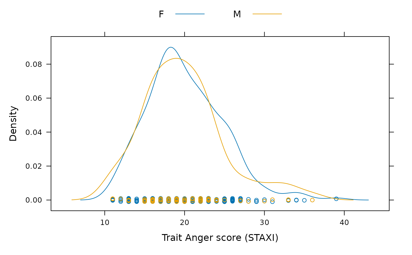
person <- unique(subset(VerbAgg, select = c(id, Gender, Anger)))
require(lattice)
densityplot(~ Anger, person, groups = Gender, auto.key = list(columns = 2),
            xlab = "Trait Anger score (STAXI)")


if(lme4:::testLevel() >= 3) { ## takes about 15 sec
    print(fmVA <- glmer(r2 ~ (Anger + Gender + btype + situ)^2 +
        (1|id) + (1|item), family = binomial, data =
       VerbAgg), corr=FALSE)
} ## testLevel() >= 3
if (interactive()) {
## much faster but less accurate
    print(fmVA0 <- glmer(r2 ~ (Anger + Gender + btype + situ)^2 +
                             (1|id) + (1|item), family = binomial,
                         data = VerbAgg, nAGQ=0L), corr=FALSE)
} ## interactive()