Fit List of lm or glm Objects with a Common Model

Fit a list of lm or glm objects with a common model for different subgroups of the data.

lmList(formula, data, family, subset, weights, na.action,
       offset, pool = !isGLM || .hasScale(family2char(family)),
       warn = TRUE, ...)

Arguments

formula: a linear formula object of the form y ~ x1+...+xn | g. In the formula object, y represents the response, x1,...,xn the covariates, and g the grouping factor specifying the partitioning of the data according to which different lm fits should be performed.
family: an optional family specification for a generalized linear model (glm).
data: an optional data frame containing the variables named in formula. By default the variables are taken from the environment from which lmer is called. See Details.
subset: an optional expression indicating the subset of the rows of data that should be used in the fit. This can be a logical vector, or a numeric vector indicating which observation numbers are to be included, or a character vector of the row names to be included. All observations are included by default.
weights: an optional vector of ‘prior weights’ to be used in the fitting process. Should be NULL or a numeric vector.
na.action: a function that indicates what should happen when the data contain NAs. The default action (na.omit, inherited from the ‘factory fresh’ value of getOption("na.action")) strips any observations with any missing values in any variables.
offset: this can be used to specify an a priori known component to be included in the linear predictor during fitting. This should be NULL or a numeric vector of length equal to the number of cases. One or more offset terms can be included in the formula instead or as well, and if more than one is specified their sum is used. See model.offset.
pool: logical scalar indicating if the variance estimate should pool the residual sums of squares. By default true if the model has a scale parameter (which includes all linear, lmer(), ones).
warn: indicating if errors in the single fits should signal a “summary” warning.
...: additional, optional arguments to be passed to the model function or family evaluation.

Value

an object of class lmList4 (see there, notably for the methods defined).

Details

While data is optional, the package authors strongly recommend its use, especially when later applying methods such as update and drop1 to the fitted model (such methods are not guaranteed to work properly if data is omitted). If data is omitted, variables will be taken from the environment of formula (if specified as a formula) or from the parent frame (if specified as a character vector).
Since lme4 version 1.1-16, if there are errors (see stop) in the single (lm() or glm()) fits, they are summarized to a warning message which is returned as attribute "warnMessage" and signalled as warning() when the warn argument is true.

In previous lme4 versions, a general (different) warning had been signalled in this case.

Examples

fm.plm  <- lmList(Reaction ~ Days | Subject, sleepstudy)
coef(fm.plm)
#>     (Intercept)      Days
#> 308    244.1927 21.764702
#> 309    205.0549  2.261785
#> 310    203.4842  6.114899
#> 330    289.6851  3.008073
#> 331    285.7390  5.266019
#> 332    264.2516  9.566768
#> 333    275.0191  9.142045
#> 334    240.1629 12.253141
#> 335    263.0347 -2.881034
#> 337    290.1041 19.025974
#> 349    215.1118 13.493933
#> 350    225.8346 19.504017
#> 351    261.1470  6.433498
#> 352    276.3721 13.566549
#> 369    254.9681 11.348109
#> 370    210.4491 18.056151
#> 371    253.6360  9.188445
#> 372    267.0448 11.298073
fm.2  <- update(fm.plm, pool = FALSE)
## coefficients are the same, "pooled or unpooled":
stopifnot( all.equal(coef(fm.2), coef(fm.plm)) )

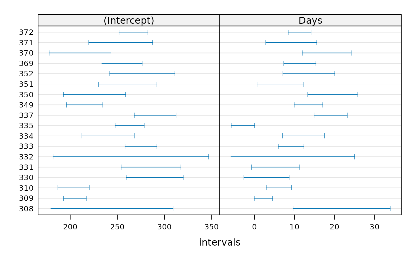
(ci <- confint(fm.plm)) # print and rather *see* :
#> An object of class "lmList4.confint"
#> , , (Intercept)
#> 
#>        2.5 %   97.5 %
#> 308 179.4339 308.9515
#> 309 193.0264 217.0834
#> 310 186.7857 220.1827
#> 330 259.4656 319.9046
#> 331 253.9831 317.4948
#> 332 181.7151 346.7882
#> 333 258.1329 291.9053
#> 334 212.3016 268.0243
#> 335 247.5990 278.4704
#> 337 267.9833 312.2249
#> 349 196.1192 234.1043
#> 350 192.8172 258.8520
#> 351 230.3022 291.9919
#> 352 241.7849 310.9592
#> 369 233.5099 276.4264
#> 370 177.7602 243.1379
#> 371 219.6541 287.6179
#> 372 251.7509 282.3387
#> 
#> , , Days
#> 
#>            2.5 %    97.5 %
#> 308  9.634266613 33.895138
#> 309  0.008641467  4.514929
#> 310  2.986982693  9.242815
#> 330 -2.652558845  8.668704
#> 331 -0.682394612 11.214432
#> 332 -5.893742346 25.027278
#> 333  5.978973800 12.305117
#> 334  7.034230035 17.472052
#> 335 -5.772399880  0.010332
#> 337 14.882372150 23.169576
#> 349  9.936302154 17.051563
#> 350 13.319294525 25.688739
#> 351  0.655729402 12.211266
#> 352  7.087781175 20.045317
#> 369  7.328617389 15.367601
#> 370 11.932968572 24.179333
#> 371  2.823051508 15.553838
#> 372  8.433264432 14.162882
#> 
plot(ci)                # how widely they vary for the individuals

Fit List of lm or glm Objects with a Common Model

Arguments

Value

Details

See also

Examples