twCoefLogitnorm

Estimating coefficients of logitnormal distribution from median and upper quantile

twCoefLogitnorm(median, quant, perc = 0.975)

Arguments

median

numeric vector: the median of the density function

quant

numeric vector: the upper quantile value

perc

numeric vector: the probability for which the quantile was specified

Value

numeric matrix with columns c("mu","sigma") rows correspond to rows in median, quant, and perc

Author

Thomas Wutzler

See also

logitnorm

Examples

# estimate the parameters, with median at 0.7 and upper quantile at 0.9
med = 0.7; upper = 0.9 
med = 0.2; upper = 0.4 
(theta <- twCoefLogitnorm(med,upper))
#>         mu      sigma 
#> -1.3862944  0.5004323 

x <- seq(0,1,length.out = 41)[-c(1,41)]  # plotting grid
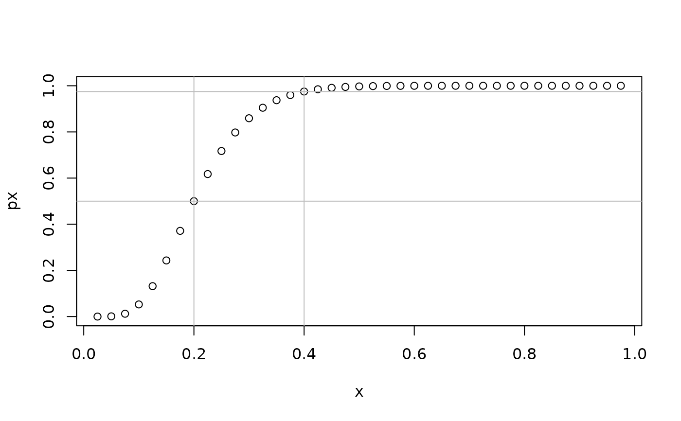
px <- plogitnorm(x,mu = theta[1],sigma = theta[2])  #percentiles function
plot(px~x); abline(v = c(med,upper),col = "gray"); abline(h = c(0.5,0.975),col = "gray")


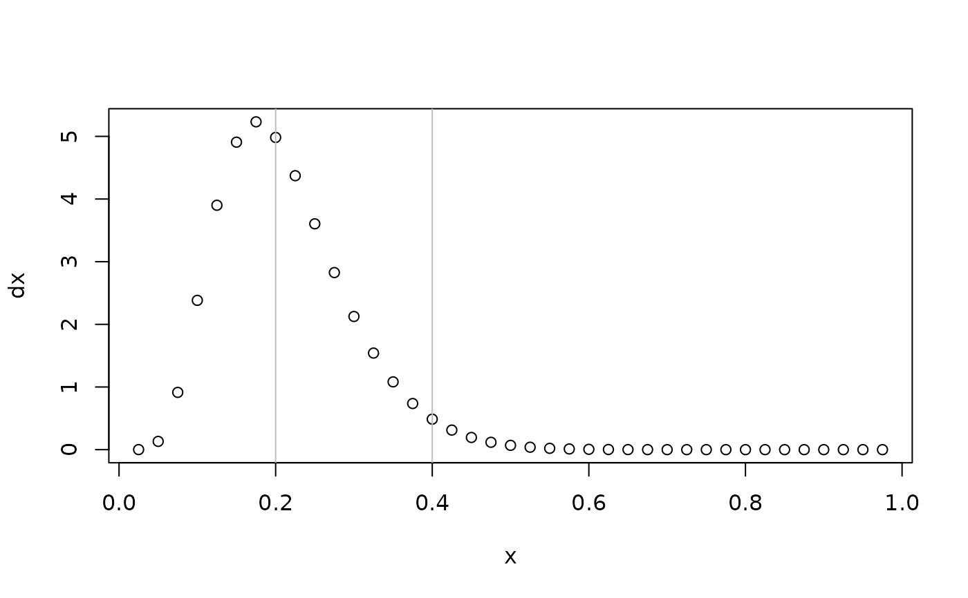
dx <- dlogitnorm(x,mu = theta[1],sigma = theta[2])  #density function
plot(dx~x); abline(v = c(med,upper),col = "gray")


# vectorized
(theta <- twCoefLogitnorm(seq(0.4,0.8,by = 0.1),0.9))
#>        mu1        mu2        mu3        mu4        mu5     sigma1     sigma2 
#> -0.4054651  0.0000000  0.4054651  0.8472979  1.3862944  1.3279273  1.1210535 
#>     sigma3     sigma4     sigma5 
#>  0.9141798  0.6887508  0.4137475 

.tmp.f <- function(){
  # xr = rlogitnorm(1e5, mu = theta["mu"], sigma = theta["sigma"])
  # median(xr)
  invlogit(theta["mu"])
  qlogitnorm(0.975, mu = theta["mu"], sigma = theta["sigma"])
}