twCoefLogitnormMLE

Estimating coefficients of logitnormal distribution from mode and upper quantile

twCoefLogitnormMLE(mle, quant, perc = 0.999)

Arguments

mle

numeric vector: the mode of the density function

quant

numeric vector: the upper quantile value

perc

numeric vector: the probability for which the quantile was specified

Value

numeric matrix with columns c("mu","sigma") rows correspond to rows in mle, quant, and perc

Author

Thomas Wutzler

See also

logitnorm

Examples

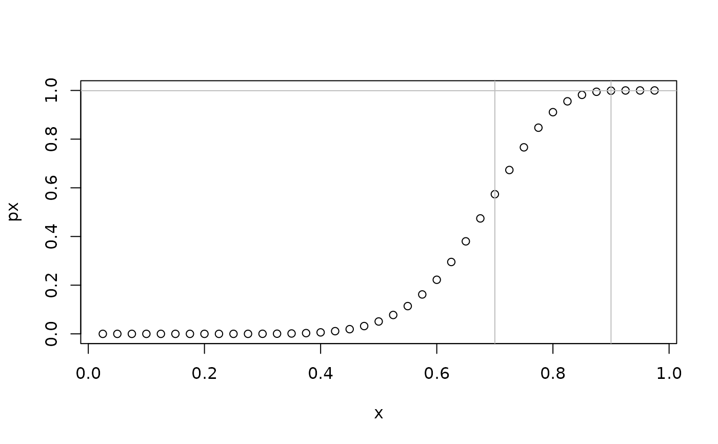
# estimate the parameters, with mode 0.7 and upper quantile 0.9
mode = 0.7; upper = 0.9
(theta <- twCoefLogitnormMLE(mode,upper))
#>             mu    sigma
#> [1,] 0.7608886 0.464783
x <- seq(0,1,length.out = 41)[-c(1,41)]  # plotting grid
px <- plogitnorm(x,mu = theta[1],sigma = theta[2])  #percentiles function
plot(px~x); abline(v = c(mode,upper),col = "gray"); abline(h = c(0.999),col = "gray")

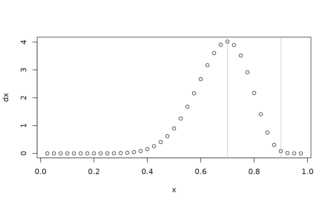
dx <- dlogitnorm(x,mu = theta[1],sigma = theta[2])  #density function
plot(dx~x); abline(v = c(mode,upper),col = "gray")

# vectorized
(theta <- twCoefLogitnormMLE(mle = seq(0.4,0.8,by = 0.1),quant = upper))
#>              mu     sigma
#> [1,] -0.2772349 0.8007190
#> [2,]  0.0000000 0.7110225
#> [3,]         NA        NA
#> [4,]         NA        NA
#> [5,]         NA        NA
# flat
(theta <- twCoefLogitnormMLEFlat(mode))
#>              mu    sigma
#> [1,] 0.01213214 1.444962