GAM censored normal family for log-normal AFT and Tobit models

Family for use with gam or bam, implementing regression for censored normal data. If $y$ is the response with mean $\mu$ and standard deviation $w^{-1/2}\exp(\theta)$, then $w^{1/2}(y-\mu)\exp(-\theta)$ follows an $N(0,1)$ distribution. That is $$y \sim N(\mu,e^{2\theta}w^{-1}).$$ $\theta$ is a single scalar for all observations. Observations may be left, interval or right censored or uncensored.

Useful for log-normal accelerated failure time (AFT) models, Tobit regression, and crudely rounded data, for example.

cnorm(theta=NULL,link="identity")

Arguments

theta: log standard deviation parameter. If supplied and positive then taken as a fixed value of standard deviation (not its log). If supplied and negative taken as negative of initial value for standard deviation (not its log).
link: The link function: "identity", "log" or "sqrt".

Value

An object of class extended.family.

Details

If the family is used with a vector response, then it is assumed that there is no censoring, and a regular Gaussian regression results. If there is censoring then the response should be supplied as a two column matrix. The first column is always numeric. Entries in the second column are as follows.

If an entry is identical to the corresponding first column entry, then it is an uncensored observation.
If an entry is numeric and different to the first column entry then there is interval censoring. The first column entry is the lower interval limit and the second column entry is the upper interval limit. $y$ is only known to be between these limits.
If the second column entry is -Inf then the observation is left censored at the value of the entry in the first column. It is only known that $y$ is less than or equal to the first column value.
If the second column entry is Inf then the observation is right censored at the value of the entry in the first column. It is only known that $y$ is greater than or equal to the first column value.

Any mixture of censored and uncensored data is allowed, but be aware that data consisting only of right and/or left censored data contain very little information.

Author

Simon N. Wood simon.wood@r-project.org

References

Wood, S.N., N. Pya and B. Saefken (2016), Smoothing parameter and model selection for general smooth models. Journal of the American Statistical Association 111, 1548-1575 doi:10.1080/01621459.2016.1180986

Examples

library(mgcv)

#######################################################
## AFT model example for colon cancer survivial data...
#######################################################

library(survival) ## for data
col1 <- colon[colon$etype==1,] ## concentrate on single event
col1$differ <- as.factor(col1$differ)
col1$sex <- as.factor(col1$sex)

## set up the AFT response... 
logt <- cbind(log(col1$time),log(col1$time))
logt[col1$status==0,2] <- Inf ## right censoring
col1$logt <- -logt ## -ve conventional for AFT versus Cox PH comparison

## fit the model...
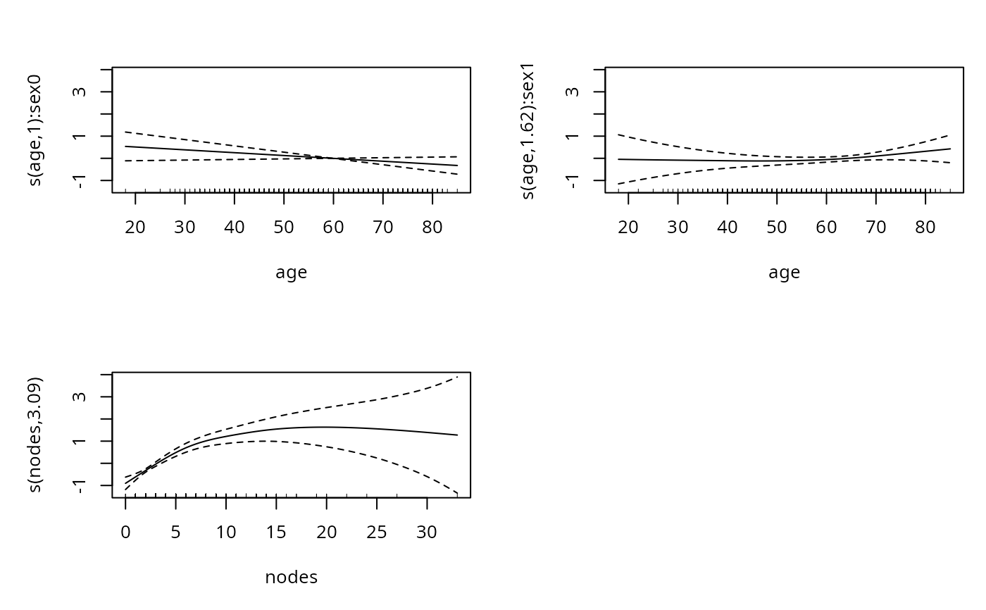
b <- gam(logt~s(age,by=sex)+sex+s(nodes)+perfor+rx+obstruct+adhere,
         family=cnorm(),data=col1)
plot(b,pages=1)   

## ... compare this to ?cox.ph

################################
## A Tobit regression example...
################################

set.seed(3);n<-400
dat <- gamSim(1,n=n)
#> Gu & Wahba 4 term additive model
ys <- dat$y - 5 ## shift data down

## truncate at zero, and set up response indicating this has happened...
y <- cbind(ys,ys)
y[ys<0,2] <- -Inf
y[ys<0,1] <- 0
dat$yt <- y
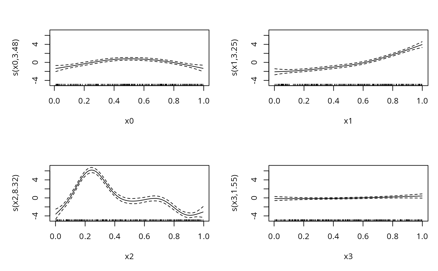
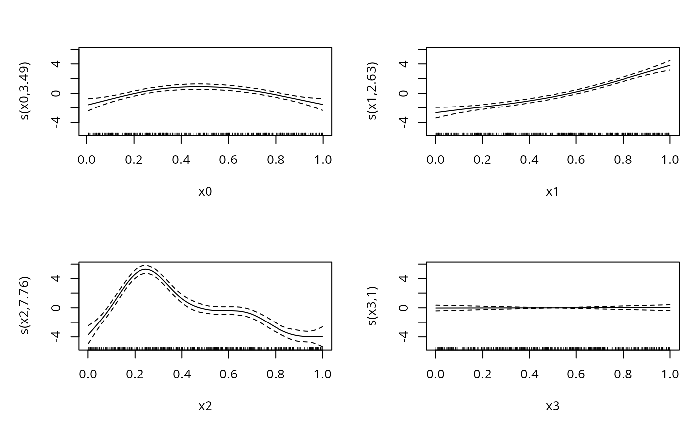
b <- gam(yt~s(x0)+s(x1)+s(x2)+s(x3),family=cnorm,data=dat)
plot(b,pages=1)


##############################
## A model for rounded data...
##############################

dat <- gamSim(1,n=n)
#> Gu & Wahba 4 term additive model
y <- round(dat$y)
y <- cbind(y-.5,y+.5) ## set up to indicate interval censoring
dat$yi <- y
b <- gam(yi~s(x0)+s(x1)+s(x2)+s(x3),family=cnorm,data=dat)
plot(b,pages=1)