Multivariate normal additive models
mvn.RdFamily for use with gam implementing smooth multivariate Gaussian regression.
The means for each dimension are given by a separate linear predictor, which may contain smooth components. Extra linear predictors may also be specified giving terms which are shared between components (see formula.gam). The Choleski factor of the response precision matrix is estimated as part of fitting.
mvn(d=2)Value
An object of class general.family.
Details
The response is d dimensional multivariate normal, where the covariance matrix is estimated,
and the means for each dimension have sperate linear predictors. Model sepcification is via a list of gam like
formulae - one for each dimension. See example.
Currently the family ignores any prior weights, and is implemented using first derivative information sufficient for BFGS estimation of smoothing parameters. "response" residuals give raw residuals, while "deviance"
residuals are standardized to be approximately independent standard normal if all is well.
References
Wood, S.N., N. Pya and B. Saefken (2016), Smoothing parameter and model selection for general smooth models. Journal of the American Statistical Association 111, 1548-1575 doi:10.1080/01621459.2016.1180986
See also
Examples
library(mgcv)
## simulate some data...
V <- matrix(c(2,1,1,2),2,2)
f0 <- function(x) 2 * sin(pi * x)
f1 <- function(x) exp(2 * x)
f2 <- function(x) 0.2 * x^11 * (10 * (1 - x))^6 + 10 *
(10 * x)^3 * (1 - x)^10
n <- 300
x0 <- runif(n);x1 <- runif(n);
x2 <- runif(n);x3 <- runif(n)
y <- matrix(0,n,2)
for (i in 1:n) {
mu <- c(f0(x0[i])+f1(x1[i]),f2(x2[i]))
y[i,] <- rmvn(1,mu,V)
}
dat <- data.frame(y0=y[,1],y1=y[,2],x0=x0,x1=x1,x2=x2,x3=x3)
## fit model...
b <- gam(list(y0~s(x0)+s(x1),y1~s(x2)+s(x3)),family=mvn(d=2),data=dat)
b
#>
#> Family: Multivariate normal
#> Link function:
#>
#> Formula:
#> y0 ~ s(x0) + s(x1)
#> <environment: 0x5efde69454f0>
#> y1 ~ s(x2) + s(x3)
#> <environment: 0x5efde69454f0>
#>
#> Estimated degrees of freedom:
#> 4.22 3.72 8.65 1.00 total = 22.59
#>
#> REML score: 472.308
summary(b)
#>
#> Family: Multivariate normal
#> Link function:
#>
#> Formula:
#> y0 ~ s(x0) + s(x1)
#> <environment: 0x5efde69454f0>
#> y1 ~ s(x2) + s(x3)
#> <environment: 0x5efde69454f0>
#>
#> Parametric coefficients:
#> Estimate Std. Error z value Pr(>|z|)
#> (Intercept) 4.53993 0.08161 55.63 <2e-16 ***
#> (Intercept).1 3.65341 0.07325 49.88 <2e-16 ***
#> ---
#> Signif. codes: 0 ‘***’ 0.001 ‘**’ 0.01 ‘*’ 0.05 ‘.’ 0.1 ‘ ’ 1
#>
#> Approximate significance of smooth terms:
#> edf Ref.df Chi.sq p-value
#> s(x0) 4.218 5.174 79.505 <2e-16 ***
#> s(x1) 3.716 4.591 773.383 <2e-16 ***
#> s.1(x2) 8.652 8.965 2161.557 <2e-16 ***
#> s.1(x3) 1.000 1.000 0.295 0.587
#> ---
#> Signif. codes: 0 ‘***’ 0.001 ‘**’ 0.01 ‘*’ 0.05 ‘.’ 0.1 ‘ ’ 1
#>
#> Deviance explained = 84%
#> -REML = 472.31 Scale est. = 1 n = 300
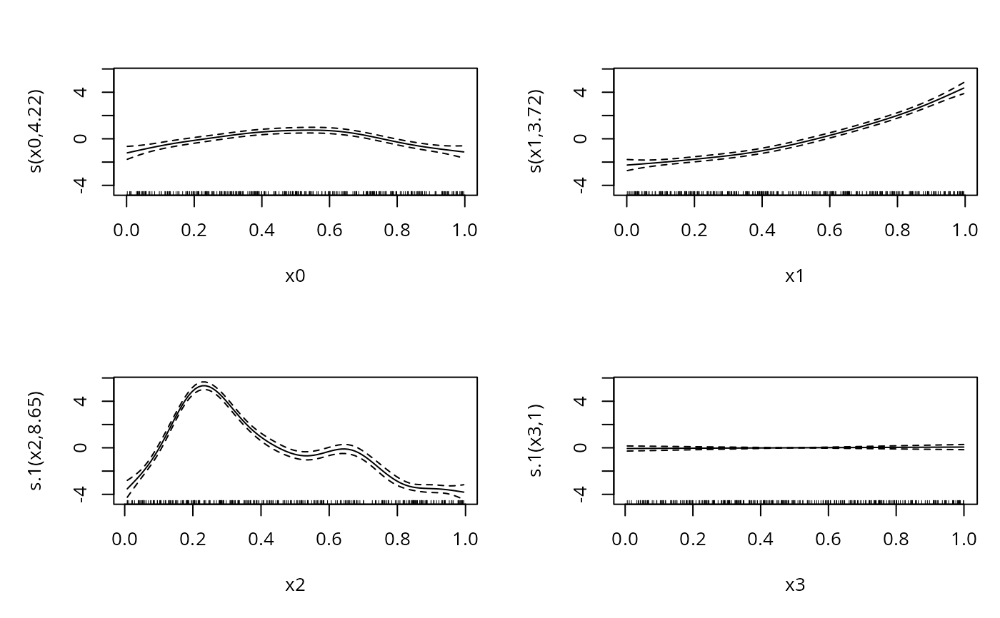
plot(b,pages=1)
 solve(crossprod(b$family$data$R)) ## estimated cov matrix
#> [,1] [,2]
#> [1,] 1.9979110 0.9910673
#> [2,] 0.9910673 1.6095367
solve(crossprod(b$family$data$R)) ## estimated cov matrix
#> [,1] [,2]
#> [1,] 1.9979110 0.9910673
#> [2,] 0.9910673 1.6095367