GAM scaled t family for heavy tailed data
scat.RdFamily for use with gam or bam, implementing regression for the heavy tailed response
variables, y, using a scaled t model. The idea is that \((y-\mu)/\sigma \sim t_\nu \) where
\(mu\) is determined by a linear predictor, while \(\sigma\) and \(\nu\) are parameters
to be estimated alongside the smoothing parameters.
scat(theta = NULL, link = "identity",min.df=3)Arguments
- theta
the parameters to be estimated \(\nu = b + \exp(\theta_1)\) (where `b' is
min.df) and \(\sigma = \exp(\theta_2)\). If supplied and both positive, then taken to be fixed values of \(\nu\) and \(\sigma\). If any negative, then absolute values taken as starting values.- link
The link function: one of
"identity","log"or"inverse".- min.df
minimum degrees of freedom. Should not be set to 2 or less as this implies infinite response variance.
Value
An object of class extended.family.
Details
Useful in place of Gaussian, when data are heavy tailed. min.df can be modified, but lower values can occasionally
lead to convergence problems in smoothing parameter estimation. In any case min.df should be >2, since only then does a t
random variable have finite variance.
References
Wood, S.N., N. Pya and B. Saefken (2016), Smoothing parameter and model selection for general smooth models. Journal of the American Statistical Association 111, 1548-1575 doi:10.1080/01621459.2016.1180986
Examples
library(mgcv)
## Simulate some t data...
set.seed(3);n<-400
dat <- gamSim(1,n=n)
#> Gu & Wahba 4 term additive model
dat$y <- dat$f + rt(n,df=4)*2
b <- gam(y~s(x0)+s(x1)+s(x2)+s(x3),family=scat(link="identity"),data=dat)
b
#>
#> Family: Scaled t(5.376,2.088)
#> Link function: identity
#>
#> Formula:
#> y ~ s(x0) + s(x1) + s(x2) + s(x3)
#>
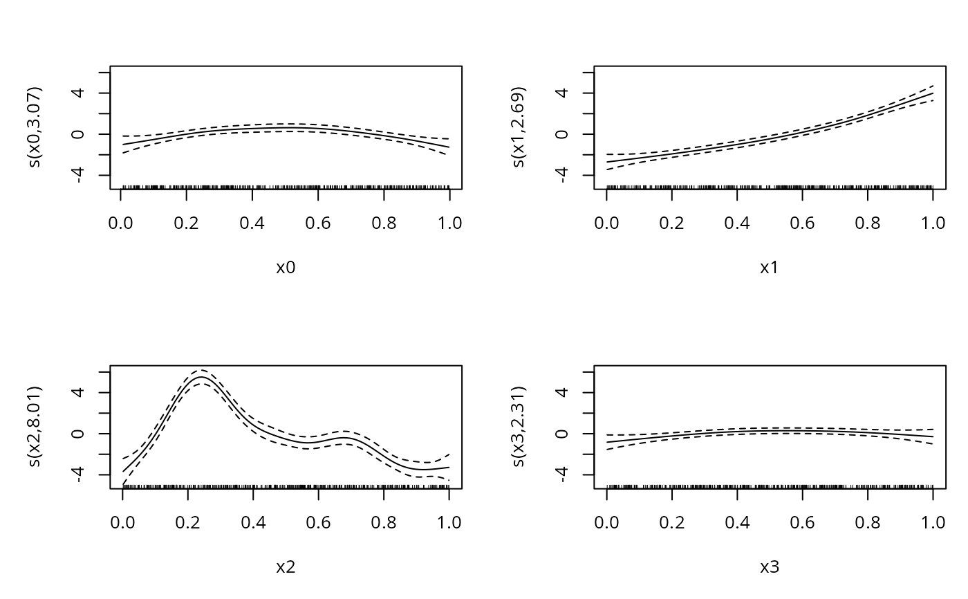
#> Estimated degrees of freedom:
#> 3.07 2.69 8.01 2.31 total = 17.08
#>
#> REML score: 961.0407
plot(b,pages=1)