Addresses NLS problems with the Levenberg-Marquardt algorithm
nls.lm.RdThe purpose of nls.lm is to minimize the sum square of the
vector returned by the function fn, by a modification of the
Levenberg-Marquardt algorithm. The user may also provide a
function jac which calculates the Jacobian.
nls.lm(par, lower=NULL, upper=NULL, fn, jac = NULL,
       control = nls.lm.control(), ...)
Arguments
- par
A list or numeric vector of starting estimates. If
paris a list, then each element must be of length 1.- lower
A numeric vector of lower bounds on each parameter. If not given, the default lower bound for each parameter is set to
-Inf.- upper
A numeric vector of upper bounds on each parameter. If not given, the default upper bound for each parameter is set to
Inf.- fn
A function that returns a vector of residuals, the sum square of which is to be minimized. The first argument of
fnmust bepar.- jac
A function to return the Jacobian for the
fnfunction.- control
An optional list of control settings. See
nls.lm.controlfor the names of the settable control values and their effect.- ...
Further arguments to be passed to
fnandjac.
Details
Both functions fn and jac (if provided) must return
numeric vectors. Length of the vector returned by fn must
not be lower than the length of par. The vector returned by
jac must have length equal to
\(length(\code{fn}(\code{par}, \dots))\cdot length(\code{par})\).
The control argument is a list; see nls.lm.control for
details.
Successful completion.
The accuracy of nls.lm is controlled by the convergence
parameters ftol, ptol, and gtol. These
parameters are used in tests which make three types of comparisons
between the approximation \(par\) and a solution
\(par_0\). nls.lm terminates when any of the tests
is satisfied. If any of the convergence parameters is less than
the machine precision, then nls.lm only attempts to satisfy
the test defined by the machine precision. Further progress is not
usually possible.
The tests assume that fn as well as jac are
reasonably well behaved. If this condition is not satisfied, then
nls.lm may incorrectly indicate convergence. The validity
of the answer can be checked, for example, by rerunning
nls.lm with tighter tolerances.
First convergence test.
If \(|z|\) denotes the Euclidean norm of a vector \(z\), then
this test attempts to guarantee that
$$|fvec| < (1 + \code{ftol})\,|fvec_0|,$$
where \(fvec_0\) denotes the result of fn function
evaluated at \(par_0\). If this condition is satisfied
with ftol \(\simeq 10^{-k}\), then the final
residual norm \(|fvec|\) has \(k\) significant decimal digits
and info is set to 1 (or to 3 if the second test is also
satisfied). Unless high precision solutions are required, the
recommended value for ftol is the square root of the machine
precision.
Second convergence test.
If \(D\) is the diagonal matrix whose entries are defined by the
array diag, then this test attempt to guarantee that
$$|D\,(par - par_0)| < \code{ptol}\,|D\,par_0|,$$
If this condition is satisfied with ptol \(\simeq
10^{-k}\), then the larger components of
\((D\,par)\) have \(k\) significant decimal digits and
info is set to 2 (or to 3 if the first test is also
satisfied). There is a danger that the smaller components of
\((D\,par)\) may have large relative errors, but if
diag is internally set, then the accuracy of the components
of \(par\) is usually related to their sensitivity. Unless high
precision solutions are required, the recommended value for
ptol is the square root of the machine precision.
Third convergence test.
This test is satisfied when the cosine of the angle between the
result of fn evaluation \(fvec\) and any column of the
Jacobian at \(par\) is at most gtol in absolute value.
There is no clear relationship between this test and the accuracy
of nls.lm, and furthermore, the test is equally well
satisfied at other critical points, namely maximizers and saddle
points. Therefore, termination caused by this test (info =
4) should be examined carefully. The recommended value for
gtol is zero.
Unsuccessful completion.
Unsuccessful termination of nls.lm can be due to improper
input parameters, arithmetic interrupts, an excessive number of
function evaluations, or an excessive number of iterations.
Improper input parameters.info is set to 0 if \(length(\code{par}) = 0\), or
\(length(fvec) < length(\code{par})\), or ftol \(< 0\),
or ptol \(< 0\), or gtol \(< 0\), or maxfev
\(\leq 0\), or factor \(\leq 0\).
Arithmetic interrupts.
If these interrupts occur in the fn function during an
early stage of the computation, they may be caused by an
unacceptable choice of \(par\) by nls.lm. In this case,
it may be possible to remedy the situation by rerunning
nls.lm with a smaller value of factor.
Excessive number of function evaluations.
A reasonable value for maxfev is \(100\cdot
(length(\code{par}) + 1)\). If the
number of calls to fn reaches maxfev, then this
indicates that the routine is converging very slowly as measured
by the progress of \(fvec\) and info is set to 5. In this
case, it may be helpful to force diag to be internally set.
Excessive number of function iterations.
The allowed number of iterations defaults to 50, can be increased if
desired.
The list returned by nls.lm has methods
for the generic functions coef,
deviance, df.residual,
print, residuals, summary,
confint,
and vcov.
Value
A list with components:
- par
The best set of parameters found.
- hessian
A symmetric matrix giving an estimate of the Hessian at the solution found.
- fvec
The result of the last
fnevaluation; that is, the residuals.- info
infois an integer code indicating the reason for termination.- 0
Improper input parameters.
- 1
Both actual and predicted relative reductions in the sum of squares are at most
ftol.- 2
Relative error between two consecutive iterates is at most
ptol.- 3
Conditions for
info= 1 andinfo= 2 both hold.- 4
The cosine of the angle between
fvecand any column of the Jacobian is at mostgtolin absolute value.- 5
Number of calls to
fnhas reachedmaxfev.- 6
ftolis too small. No further reduction in the sum of squares is possible.- 7
ptolis too small. No further improvement in the approximate solutionparis possible.- 8
gtolis too small.fvecis orthogonal to the columns of the Jacobian to machine precision.- 9
The number of iterations has reached
maxiter.
- message
character string indicating reason for termination
.
- diag
The result list of
diag. See Details.- niter
The number of iterations completed before termination.
- rsstrace
The residual sum of squares at each iteration. Can be used to check the progress each iteration.
- deviance
The sum of the squared residual vector.
References
J.J. Moré, "The Levenberg-Marquardt algorithm: implementation and theory," in Lecture Notes in Mathematics 630: Numerical Analysis, G.A. Watson (Ed.), Springer-Verlag: Berlin, 1978, pp. 105-116.
Note
The public domain FORTRAN sources of MINPACK package by J.J. Moré, implementing the Levenberg-Marquardt algorithm were downloaded from https://netlib.org/minpack/, and left unchanged. The contents of this manual page are largely extracted from the comments of MINPACK sources.
See also
Examples
###### example 1
## values over which to simulate data
x <- seq(0,5,length=100)
## model based on a list of parameters
getPred <- function(parS, xx) parS$a * exp(xx * parS$b) + parS$c
## parameter values used to simulate data
pp <- list(a=9,b=-1, c=6)
## simulated data, with noise
simDNoisy <- getPred(pp,x) + rnorm(length(x),sd=.1)
## plot data
plot(x,simDNoisy, main="data")
## residual function
residFun <- function(p, observed, xx) observed - getPred(p,xx)
## starting values for parameters
parStart <- list(a=3,b=-.001, c=1)
## perform fit
nls.out <- nls.lm(par=parStart, fn = residFun, observed = simDNoisy,
xx = x, control = nls.lm.control(nprint=1))
#> It. 0, RSS = 1970.11, Par. = 3 -0.001 1
#> It. 1, RSS = 323.071, Par. = 5.25248 -0.148204 3.23758
#> It. 2, RSS = 102.039, Par. = 6.67342 -0.303727 4.26888
#> It. 3, RSS = 52.313, Par. = 7.44748 -0.419686 4.69814
#> It. 4, RSS = 32.2883, Par. = 7.57229 -0.70388 6.11152
#> It. 5, RSS = 3.52944, Par. = 8.60238 -1.01278 6.24134
#> It. 6, RSS = 1.04618, Par. = 8.91898 -1.00262 6.02861
#> It. 7, RSS = 1.0461, Par. = 8.91932 -1.00311 6.02862
#> It. 8, RSS = 1.0461, Par. = 8.91931 -1.00311 6.02861
## plot model evaluated at final parameter estimates
lines(x,getPred(as.list(coef(nls.out)), x), col=2, lwd=2)
 ## summary information on parameter estimates
summary(nls.out)
#>
#> Parameters:
#> Estimate Std. Error t value Pr(>|t|)
#> a 8.91931 0.04471 199.5 <2e-16 ***
#> b -1.00311 0.01099 -91.3 <2e-16 ***
#> c 6.02861 0.02010 300.0 <2e-16 ***
#> ---
#> Signif. codes: 0 ‘***’ 0.001 ‘**’ 0.01 ‘*’ 0.05 ‘.’ 0.1 ‘ ’ 1
#>
#> Residual standard error: 0.1038 on 97 degrees of freedom
#> Number of iterations to termination: 8
#> Reason for termination: Relative error in the sum of squares is at most `ftol'.
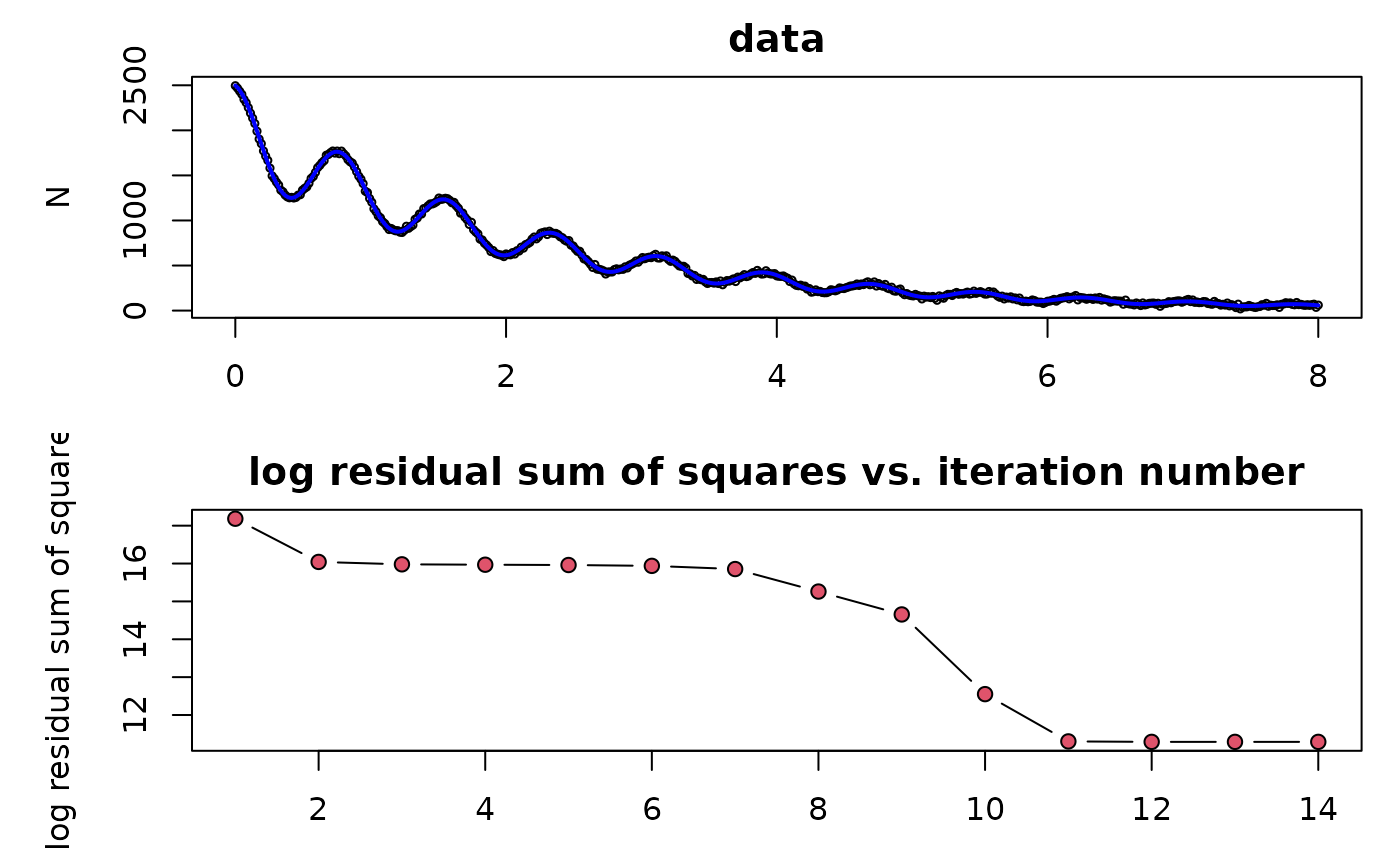
###### example 2
## function to simulate data
f <- function(TT, tau, N0, a, f0) {
expr <- expression(N0*exp(-TT/tau)*(1 + a*cos(f0*TT)))
eval(expr)
}
## helper function for an analytical gradient
j <- function(TT, tau, N0, a, f0) {
expr <- expression(N0*exp(-TT/tau)*(1 + a*cos(f0*TT)))
c(eval(D(expr, "tau")), eval(D(expr, "N0" )),
eval(D(expr, "a" )), eval(D(expr, "f0" )))
}
## values over which to simulate data
TT <- seq(0, 8, length=501)
## parameter values underlying simulated data
p <- c(tau = 2.2, N0 = 1000, a = 0.25, f0 = 8)
## get data
Ndet <- do.call("f", c(list(TT = TT), as.list(p)))
## with noise
N <- Ndet + rnorm(length(Ndet), mean=Ndet, sd=.01*max(Ndet))
## plot the data to fit
par(mfrow=c(2,1), mar = c(3,5,2,1))
plot(TT, N, bg = "black", cex = 0.5, main="data")
## define a residual function
fcn <- function(p, TT, N, fcall, jcall)
(N - do.call("fcall", c(list(TT = TT), as.list(p))))
## define analytical expression for the gradient
fcn.jac <- function(p, TT, N, fcall, jcall)
-do.call("jcall", c(list(TT = TT), as.list(p)))
## starting values
guess <- c(tau = 2.2, N0 = 1500, a = 0.25, f0 = 10)
## to use an analytical expression for the gradient found in fcn.jac
## uncomment jac = fcn.jac
out <- nls.lm(par = guess, fn = fcn, jac = fcn.jac,
fcall = f, jcall = j,
TT = TT, N = N, control = nls.lm.control(nprint=1))
#> It. 0, RSS = 2.90164e+07, Par. = 2.2 1500 0.25 10
#> It. 1, RSS = 9.27337e+06, Par. = 2.10933 2039.81 -0.0269788 9.91506
#> It. 2, RSS = 8.70172e+06, Par. = 2.17455 2020.06 0.0490791 10.6412
#> It. 3, RSS = 8.61416e+06, Par. = 2.16353 2026.68 0.027969 10.4777
#> It. 4, RSS = 8.54584e+06, Par. = 2.16563 2025.62 0.0312413 10.1612
#> It. 5, RSS = 8.35615e+06, Par. = 2.16559 2025.37 0.0388 9.74136
#> It. 6, RSS = 7.68212e+06, Par. = 2.16466 2025.13 0.0553991 9.1744
#> It. 7, RSS = 4.24015e+06, Par. = 2.16372 2023.91 0.0960988 8.36641
#> It. 8, RSS = 2.31672e+06, Par. = 2.18495 2008.86 0.215268 7.63573
#> It. 9, RSS = 282481, Par. = 2.17181 2015.01 0.2142 7.96673
#> It. 10, RSS = 81059, Par. = 2.20249 1999.57 0.248835 8.00931
#> It. 11, RSS = 80062.4, Par. = 2.20299 1999.55 0.249231 8.00235
#> It. 12, RSS = 80062.2, Par. = 2.20302 1999.54 0.249246 8.00244
#> It. 13, RSS = 80062.2, Par. = 2.20302 1999.54 0.249246 8.00244
## get the fitted values
N1 <- do.call("f", c(list(TT = TT), out$par))
## add a blue line representing the fitting values to the plot of data
lines(TT, N1, col="blue", lwd=2)
## add a plot of the log residual sum of squares as it is made to
## decrease each iteration; note that the RSS at the starting parameter
## values is also stored
plot(1:(out$niter+1), log(out$rsstrace), type="b",
main="log residual sum of squares vs. iteration number",
xlab="iteration", ylab="log residual sum of squares", pch=21,bg=2)
## summary information on parameter estimates
summary(nls.out)
#>
#> Parameters:
#> Estimate Std. Error t value Pr(>|t|)
#> a 8.91931 0.04471 199.5 <2e-16 ***
#> b -1.00311 0.01099 -91.3 <2e-16 ***
#> c 6.02861 0.02010 300.0 <2e-16 ***
#> ---
#> Signif. codes: 0 ‘***’ 0.001 ‘**’ 0.01 ‘*’ 0.05 ‘.’ 0.1 ‘ ’ 1
#>
#> Residual standard error: 0.1038 on 97 degrees of freedom
#> Number of iterations to termination: 8
#> Reason for termination: Relative error in the sum of squares is at most `ftol'.
###### example 2
## function to simulate data
f <- function(TT, tau, N0, a, f0) {
expr <- expression(N0*exp(-TT/tau)*(1 + a*cos(f0*TT)))
eval(expr)
}
## helper function for an analytical gradient
j <- function(TT, tau, N0, a, f0) {
expr <- expression(N0*exp(-TT/tau)*(1 + a*cos(f0*TT)))
c(eval(D(expr, "tau")), eval(D(expr, "N0" )),
eval(D(expr, "a" )), eval(D(expr, "f0" )))
}
## values over which to simulate data
TT <- seq(0, 8, length=501)
## parameter values underlying simulated data
p <- c(tau = 2.2, N0 = 1000, a = 0.25, f0 = 8)
## get data
Ndet <- do.call("f", c(list(TT = TT), as.list(p)))
## with noise
N <- Ndet + rnorm(length(Ndet), mean=Ndet, sd=.01*max(Ndet))
## plot the data to fit
par(mfrow=c(2,1), mar = c(3,5,2,1))
plot(TT, N, bg = "black", cex = 0.5, main="data")
## define a residual function
fcn <- function(p, TT, N, fcall, jcall)
(N - do.call("fcall", c(list(TT = TT), as.list(p))))
## define analytical expression for the gradient
fcn.jac <- function(p, TT, N, fcall, jcall)
-do.call("jcall", c(list(TT = TT), as.list(p)))
## starting values
guess <- c(tau = 2.2, N0 = 1500, a = 0.25, f0 = 10)
## to use an analytical expression for the gradient found in fcn.jac
## uncomment jac = fcn.jac
out <- nls.lm(par = guess, fn = fcn, jac = fcn.jac,
fcall = f, jcall = j,
TT = TT, N = N, control = nls.lm.control(nprint=1))
#> It. 0, RSS = 2.90164e+07, Par. = 2.2 1500 0.25 10
#> It. 1, RSS = 9.27337e+06, Par. = 2.10933 2039.81 -0.0269788 9.91506
#> It. 2, RSS = 8.70172e+06, Par. = 2.17455 2020.06 0.0490791 10.6412
#> It. 3, RSS = 8.61416e+06, Par. = 2.16353 2026.68 0.027969 10.4777
#> It. 4, RSS = 8.54584e+06, Par. = 2.16563 2025.62 0.0312413 10.1612
#> It. 5, RSS = 8.35615e+06, Par. = 2.16559 2025.37 0.0388 9.74136
#> It. 6, RSS = 7.68212e+06, Par. = 2.16466 2025.13 0.0553991 9.1744
#> It. 7, RSS = 4.24015e+06, Par. = 2.16372 2023.91 0.0960988 8.36641
#> It. 8, RSS = 2.31672e+06, Par. = 2.18495 2008.86 0.215268 7.63573
#> It. 9, RSS = 282481, Par. = 2.17181 2015.01 0.2142 7.96673
#> It. 10, RSS = 81059, Par. = 2.20249 1999.57 0.248835 8.00931
#> It. 11, RSS = 80062.4, Par. = 2.20299 1999.55 0.249231 8.00235
#> It. 12, RSS = 80062.2, Par. = 2.20302 1999.54 0.249246 8.00244
#> It. 13, RSS = 80062.2, Par. = 2.20302 1999.54 0.249246 8.00244
## get the fitted values
N1 <- do.call("f", c(list(TT = TT), out$par))
## add a blue line representing the fitting values to the plot of data
lines(TT, N1, col="blue", lwd=2)
## add a plot of the log residual sum of squares as it is made to
## decrease each iteration; note that the RSS at the starting parameter
## values is also stored
plot(1:(out$niter+1), log(out$rsstrace), type="b",
main="log residual sum of squares vs. iteration number",
xlab="iteration", ylab="log residual sum of squares", pch=21,bg=2)
 ## get information regarding standard errors
summary(out)
#>
#> Parameters:
#> Estimate Std. Error t value Pr(>|t|)
#> tau 2.203e+00 3.336e-03 660.4 <2e-16 ***
#> N0 2.000e+03 2.129e+00 939.2 <2e-16 ***
#> a 2.492e-01 1.096e-03 227.4 <2e-16 ***
#> f0 8.002e+00 2.822e-03 2836.0 <2e-16 ***
#> ---
#> Signif. codes: 0 ‘***’ 0.001 ‘**’ 0.01 ‘*’ 0.05 ‘.’ 0.1 ‘ ’ 1
#>
#> Residual standard error: 12.69 on 497 degrees of freedom
#> Number of iterations to termination: 13
#> Reason for termination: Relative error in the sum of squares is at most `ftol'.
## get information regarding standard errors
summary(out)
#>
#> Parameters:
#> Estimate Std. Error t value Pr(>|t|)
#> tau 2.203e+00 3.336e-03 660.4 <2e-16 ***
#> N0 2.000e+03 2.129e+00 939.2 <2e-16 ***
#> a 2.492e-01 1.096e-03 227.4 <2e-16 ***
#> f0 8.002e+00 2.822e-03 2836.0 <2e-16 ***
#> ---
#> Signif. codes: 0 ‘***’ 0.001 ‘**’ 0.01 ‘*’ 0.05 ‘.’ 0.1 ‘ ’ 1
#>
#> Residual standard error: 12.69 on 497 degrees of freedom
#> Number of iterations to termination: 13
#> Reason for termination: Relative error in the sum of squares is at most `ftol'.