Pharmacokinetics of Cefamandole

The Cefamandole data frame has 84 rows and 3 columns.

Format

This data frame contains the following columns:

Subject

a factor giving the subject from which the sample was drawn.

Time

a numeric vector giving the time at which the sample was drawn (minutes post-injection).

conc

a numeric vector giving the observed plasma concentration of cefamandole (mcg/ml).

Details

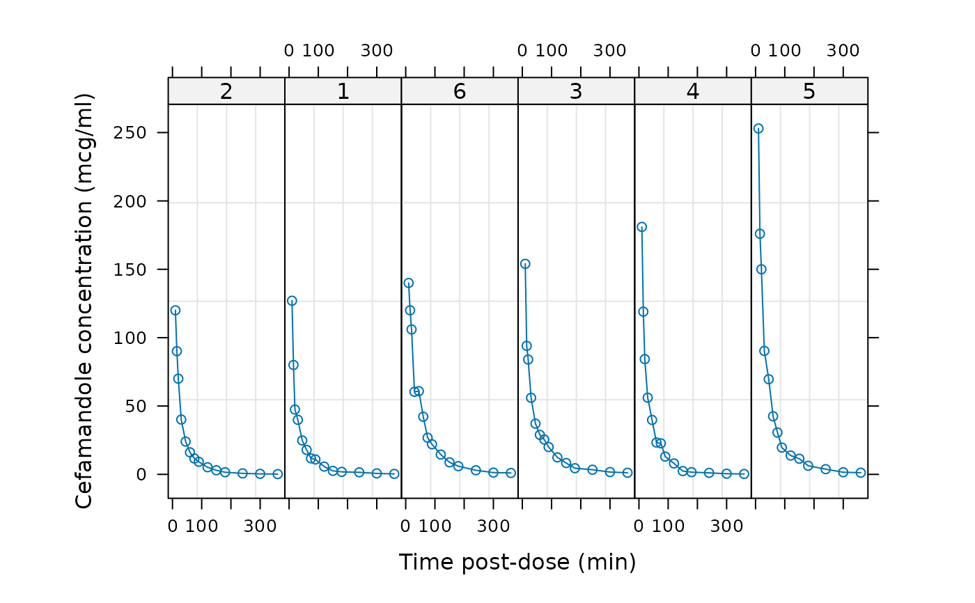
Davidian and Giltinan (1995, 1.1, p. 2) describe data obtained during a pilot study to investigate the pharmacokinetics of the drug cefamandole. Plasma concentrations of the drug were measured on six healthy volunteers at 14 time points following an intraveneous dose of 15 mg/kg body weight of cefamandole.

Source

Pinheiro, J. C. and Bates, D. M. (2000), Mixed-Effects Models in S and S-PLUS, Springer, New York. (Appendix A.4)

Davidian, M. and Giltinan, D. M. (1995), Nonlinear Models for Repeated Measurement Data, Chapman and Hall, London.

Examples

plot(Cefamandole)

fm1 <- nlsList(SSbiexp, data = Cefamandole)
summary(fm1)
#> Call:
#>   Model: conc ~ SSbiexp(Time, A1, lrc1, A2, lrc2) | Subject 
#>    Data: Cefamandole 
#> 
#> Coefficients:
#>    A1 
#>   Estimate Std. Error  t value     Pr(>|t|)
#> 2 191.3341   21.38625 8.946595 2.800684e-12
#> 1 497.5333  170.10972 2.924779 2.227380e-03
#> 6 121.7071   22.08024 5.512036 4.938589e-03
#> 3 460.8836  137.08512 3.362025 7.081633e-03
#> 4 485.3220   99.84752 4.860631 1.699109e-06
#> 5 411.5147   51.41634 8.003579 1.513503e-04
#>    lrc1 
#>    Estimate Std. Error    t value     Pr(>|t|)
#> 2 -2.599155  0.2354814 -11.037623 3.463458e-13
#> 1 -1.674042  0.2283020  -7.332577 1.302103e-06
#> 6 -2.597524  0.3801661  -6.832603 1.237735e-03
#> 3 -1.728710  0.2037836  -8.483070 6.814224e-06
#> 4 -1.852475  0.1850105 -10.012806 1.725950e-09
#> 5 -2.085231  0.1729003 -12.060312 4.629005e-06
#>    A2 
#>    Estimate Std. Error  t value     Pr(>|t|)
#> 2  34.39548   26.19982 1.312814 1.852725e-04
#> 1  63.07492   14.67306 4.298690 1.336682e-04
#> 6  99.12318   27.69506 3.579093 4.202739e-02
#> 3  88.41797   11.82932 7.474474 2.063732e-05
#> 4  99.60164   18.89437 5.271499 8.044466e-07
#> 5 164.78474   24.35931 6.764755 5.489025e-04
#>    lrc2 
#>    Estimate Std. Error    t value     Pr(>|t|)
#> 2 -4.160739  0.5475810  -7.598398 1.417916e-11
#> 1 -3.883162  0.2081573 -18.654939 1.629855e-10
#> 6 -4.132324  0.1965967 -21.019294 8.412511e-08
#> 3 -4.070260  0.1316273 -30.922612 2.839152e-11
#> 4 -3.826142  0.1533673 -24.947574 2.049709e-13
#> 5 -3.832660  0.1086349 -35.280209 1.629080e-10
#> 
#> Residual standard error: 3.815833 on 60 degrees of freedom
#>