Common Data and Absolute Intervals Returned by Plot Methods
np_plot_data.RdBias-corrected bounds are experimental (pre-beta research), incomplete, and not recommended for general-purpose inference. See the experimental-status section below.
Plot methods return an np_plot_data object for output="data"
or output="plot-data". It contains plotted targets and geometry, not
fitted estimator objects. These methods inspect, extract or replay that data
without fitting, bandwidth selection, bootstrap simulation or RNG use.
Usage
# S3 method for class 'np_plot_data'
print(x, ...)
# S3 method for class 'np_plot_data'
as.data.frame(x, row.names = NULL, optional = FALSE,
  panel = NULL, target = NULL, band = NULL, ...)
# S3 method for class 'np_plot_data'
plot(x, y = NULL, ..., panel = NULL, target = NULL,
  band = NULL, renderer = c("base", "rgl"))
Arguments
- x
A plot-data object.
- y
Unused; must be
NULL.- panel
Panel identifier or one-based index. Extraction requires an explicit selection when there is more than one panel. Replay defaults to all panels.
- target
Scalar target identifier or one-based index within the selected panel. Extraction requires a selection when multiple targets exist, for example several quantiles or derivative components. Replay defaults to all targets.
- band
An available band name. Extraction requires a selection if several bands were computed. Replay defaults to all computed bands. This selects saved endpoints; it never computes a missing band.
- renderer
Base graphics or the existing interactive rgl surface renderer. One-dimensional, coefficient, contour and image replay use base graphics.
- row.names, optional
Standard data-frame method arguments.
optionalis accepted for generic compatibility; column names remain the schema names.- ...
Graphical overrides for replay, unused by
print. Additional extraction arguments are rejected.
Details
All families use the same endpoint convention: lower and upper
are absolute values on the target scale. Do not add the estimate or corrected
estimate to them. The corrected estimate need not be the interval midpoint,
particularly for percentile constructions. A standard error is a genuine
available SE, never an interval width divided by a critical value; its reference
is identified in the corresponding inference record. Unavailable values remain
NA with explicit status and their evaluation rows are retained.
The object has these components:
- schema_version
Integer schema identifier, currently
1L.- family
Estimator family name.
- request
Resolved plot controls and, where applicable, explicitly supplied argument names. These describe the computation; changing them does not recompute it.
- panels
Named panels. Each contains
grid,variables,values,intervalsanddisplay. Grid columns have stable identifierseval_1,eval_2, etc., avoiding collisions with target field names.variablesmaps each coordinate to its original name, role and label, preserving factor/ordered grid columns. Values are keyed byrow_idandtarget_id, withestimate,bias_corrected,std_errorandstatus. Intervals addband,alpha,lower,upper,family_idandstatus. Display holds only retained plotting geometry and styles, including requested observations, rugs or bootstrap boxplot summaries.- targets
Scalar target identities, quantities, labels, derivative variables and orders, multi-indices, coefficient terms, response levels and quantile
tauvalues where relevant.inference_idlinks to method metadata.- inference
Compact records of the actual construction, law, calibration, SE reference, projection and available resolution diagnostics. Categorical contrast metadata records the lower and upper comparison levels for every grid row, with orientation
upper minus lower. Full bootstrap draws, covariance workspaces, fitted models and RNG states are not plot results.- coverage_families
The finite-grid event and its explicit panel/row/target members. Pointwise intervals do not imply joint coverage. Simultaneous and Bonferroni scopes remain those of the selected method; panels, derivatives and quantiles are not combined unless that method actually calibrated their union. No coverage between grid points is implied.
- diagnostics
Additional plot-result diagnostics when available.
Coefficient displays of plus/minus one standard error use band "std_error",
alpha=NA, status "display_only" and no confidence-family claim.
For class-probability plots, rows padded for missing evaluation coordinates
remain in the display grid but are excluded from coverage families and
Bonferroni counts. Defined targets with unavailable uncertainty remain family
members; an unavailable interval does not silently reduce the requested family.
An empirical copula probability-pair display likewise has no estimated target or interval. Asking for a missing band is an error.
data and plot-data return the same numerical payload under matched
controls; only the latter draws the original estimator plot. plot(x) on
saved plot data replays its geometry. It does not recompute inferential quantities
or acquire missing fitted state. The original estimator methods retain their
existing annotations and graphical controls.
The schema deliberately replaces plot-only d1/r1/cd1
objects, signed error slots, width arrays and inherited estimator methods.
Fitted-model APIs and control-constructor arguments are unchanged. For plot
arguments, use snake_case spellings such as boot_control,
bias_control, gaussian_draws and gradient_order.
Value
as.data.frame returns the selected grid and values joined to the selected
absolute interval columns. Interval status is named interval_status in
this flattened table. Without intervals it returns only coordinates and values.
print invisibly returns x. Base replay invisibly returns NULL;
interactive surface replay returns the renderer's widget.
Experimental status of bias-corrected inference
All bias-corrected confidence intervals and bands are experimental (pre-beta research), incomplete, and not recommended for general-purpose inference. This status remains in effect unless the documentation explicitly states otherwise for a particular method and scope. It applies wherever bias-corrected bounds are available: asymptotic and bootstrap constructions, including legacy methods, pointwise intervals, Bonferroni intervals and simultaneous bands, for levels and supported derivatives.
These methods form an ongoing research project. Implementation support, numerical checks and favorable simulation results in selected settings do not establish generally valid coverage. Coverage can fail outside the studied settings, and available options do not constitute a general solution to bias-corrected inference. Method-specific assumptions, restrictions and known failures must be considered when experimenting with these bounds.
Examples
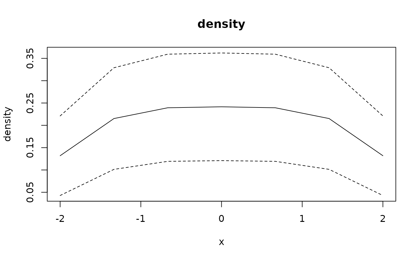
x <- seq(-2, 2, length.out = 30)
bw <- npudensbw(dat = data.frame(x = x), bws = .6,
                bandwidth.compute = FALSE)
p <- plot(bw, errors = "asymptotic", band = "pointwise",
          neval = 7, output = "data")
d <- as.data.frame(p)
d[c("eval_1", "estimate", "lower", "upper")]
#>       eval_1  estimate      lower     upper
#> 1 -2.0000000 0.1319151 0.04279888 0.2210312
#> 2 -1.3333333 0.2151848 0.10136569 0.3290039
#> 3 -0.6666667 0.2393504 0.11931028 0.3593905
#> 4  0.0000000 0.2415341 0.12094763 0.3621206
#> 5  0.6666667 0.2393504 0.11931028 0.3593905
#> 6  1.3333333 0.2151848 0.10136569 0.3290039
#> 7  2.0000000 0.1319151 0.04279888 0.2210312
p$targets
#>   target_id quantity   label variable level term inference_id tau order
#> 1  target_1  density density     <NA>  <NA> <NA>  inference_1  NA    NA
#>   multi_index
#> 1
p$panels[[1]]$variables
#>   coordinate name role label
#> 1     eval_1    x    X     x
plot(p)