Determines the power, the non-centrality parameter, or the degrees of freedom for the lambda-prime distribution with (optional) Type 1 and Type 2 error plots.
Usage
power.lp.test(
  power = NULL,
  ncp = NULL,
  req.sign = "+",
  null.ncp = 0,
  df = NULL,
  alpha = 0.05,
  alternative = c("two.sided", "one.sided", "two.one.sided"),
  plot = TRUE,
  verbose = 1,
  utf = FALSE
)
Arguments
- power
statistical power \((1 - \beta)\); either
power,ncpordfneeds to be NULL (and is then estimated).- ncp
non-centrality parameter for the alternative; either
power,ncpordfneeds to be NULL (and is then estimated).- req.sign
whether
ncpis expected to be greater '+1', less than '-1', or within '0' thenull.ncpbounds; only relevant ifncpis to be estimated.- null.ncp
non-centrality parameter for the null. When alternative = "two.one.sided", the function expects two values in the form
c(lower, upper). If a single value is provided, it is interpreted as the absolute bound and automatically expanded toc(-value, +value).- df
degrees of freedom; either
power,ncpordfneeds to be NULL (and is then estimated).- alpha
type 1 error rate, defined as the probability of incorrectly rejecting a true null hypothesis, denoted as \(\alpha\).
- alternative
character; the direction or type of the hypothesis test: "two.sided", "one.sided", or "two.one.sided". "two.one.sided" is used for equivalence and minimal effect testing.
- plot
logical;
FALSEswitches off Type 1 and Type 2 error plot.TRUEby default.- verbose
1by default (returns test, hypotheses, and results), if2a more detailed output is given (plus key parameters and definitions), if0no output is printed on the console.- utf
logical; whether the output should show Unicode characters (if encoding allows for it).
FALSEby default.
Value
- power
statistical power \((1 - \beta)\).
- ncp
non-centrality parameter under alternative.
- null.ncp
non-centrality parameter under null.
- df
degrees of freedom.
- alpha
type 1 error rate (user-specified).
- alternative
the direction or type of the hypothesis test.
- t.alpha
critical value(s).
- beta
type 2 error rate.
- type.s
type S error rate (only for two-tailed test).
- type.m
type M error rate (only for two-tailed test).
Examples
# two-sided
# power defined as the probability of observing test statistics greater
# than the positive critical value OR less than the negative critical value
power.lp.test(ncp = 1.960, df = 100, alpha = 0.05,
alternative = "two.sided", plot = FALSE)
#> +--------------------------------------------------+
#> | POWER CALCULATION |
#> +--------------------------------------------------+
#>
#> Generic Lambda-Prime Distribution
#>
#> ----------------------------------------------------
#> Hypotheses
#> ----------------------------------------------------
#> H0 (Null) : lambda = null.lambda
#> H1 (Alternative) : lambda != null.lambda
#>
#> ----------------------------------------------------
#> Results
#> ----------------------------------------------------
#> Target NCP (lambda) = 1.960 (vs. null.lambda = 0)
#> Degrees of Freedom = 100
#> Type 1 Error (alpha) = 0.050
#> Type 2 Error (beta) = 0.502
#> Statistical Power = 0.498 <<
#>
power.lp.test(power = 0.800, df = 100, alpha = 0.05,
alternative = "two.sided", plot = FALSE)
#> +--------------------------------------------------+
#> | MINIMUM DETECTABLE NCP CALCULATION |
#> +--------------------------------------------------+
#>
#> Generic Lambda-Prime Distribution
#>
#> ----------------------------------------------------
#> Hypotheses
#> ----------------------------------------------------
#> H0 (Null) : lambda = null.lambda
#> H1 (Alternative) : lambda != null.lambda
#>
#> ----------------------------------------------------
#> Results
#> ----------------------------------------------------
#> Target NCP (lambda) = 2.825 (vs. null.lambda = 0) <<
#> Degrees of Freedom = 100
#> Type 1 Error (alpha) = 0.050
#> Type 2 Error (beta) = 0.200
#> Statistical Power = 0.800
#>
# the two examples below estimate the df's based upon the first example
# (revealing a power of 0.498; df = 94.11) and the second example (revealing
# a ncp of 2.825; df = 101.06)
power.lp.test(ncp = 1.960, power = 0.498, alpha = 0.05,
alternative = "two.sided", plot = FALSE)
#> +--------------------------------------------------+
#> | SAMPLE SIZE CALCULATION |
#> +--------------------------------------------------+
#>
#> Generic Lambda-Prime Distribution
#>
#> ----------------------------------------------------
#> Hypotheses
#> ----------------------------------------------------
#> H0 (Null) : lambda = null.lambda
#> H1 (Alternative) : lambda != null.lambda
#>
#> ----------------------------------------------------
#> Results
#> ----------------------------------------------------
#> Target NCP (lambda) = 1.960 (vs. null.lambda = 0)
#> Degrees of Freedom = 94.11 <<
#> Type 1 Error (alpha) = 0.050
#> Type 2 Error (beta) = 0.502
#> Statistical Power = 0.498
#>
power.lp.test(ncp = 2.825, power = 0.800, alpha = 0.05,
alternative = "two.sided", plot = FALSE)
#> +--------------------------------------------------+
#> | SAMPLE SIZE CALCULATION |
#> +--------------------------------------------------+
#>
#> Generic Lambda-Prime Distribution
#>
#> ----------------------------------------------------
#> Hypotheses
#> ----------------------------------------------------
#> H0 (Null) : lambda = null.lambda
#> H1 (Alternative) : lambda != null.lambda
#>
#> ----------------------------------------------------
#> Results
#> ----------------------------------------------------
#> Target NCP (lambda) = 2.825 (vs. null.lambda = 0)
#> Degrees of Freedom = 101.06 <<
#> Type 1 Error (alpha) = 0.050
#> Type 2 Error (beta) = 0.200
#> Statistical Power = 0.800
#>
# one-sided
# power is defined as the probability of observing a test statistic greater
# than the critical value
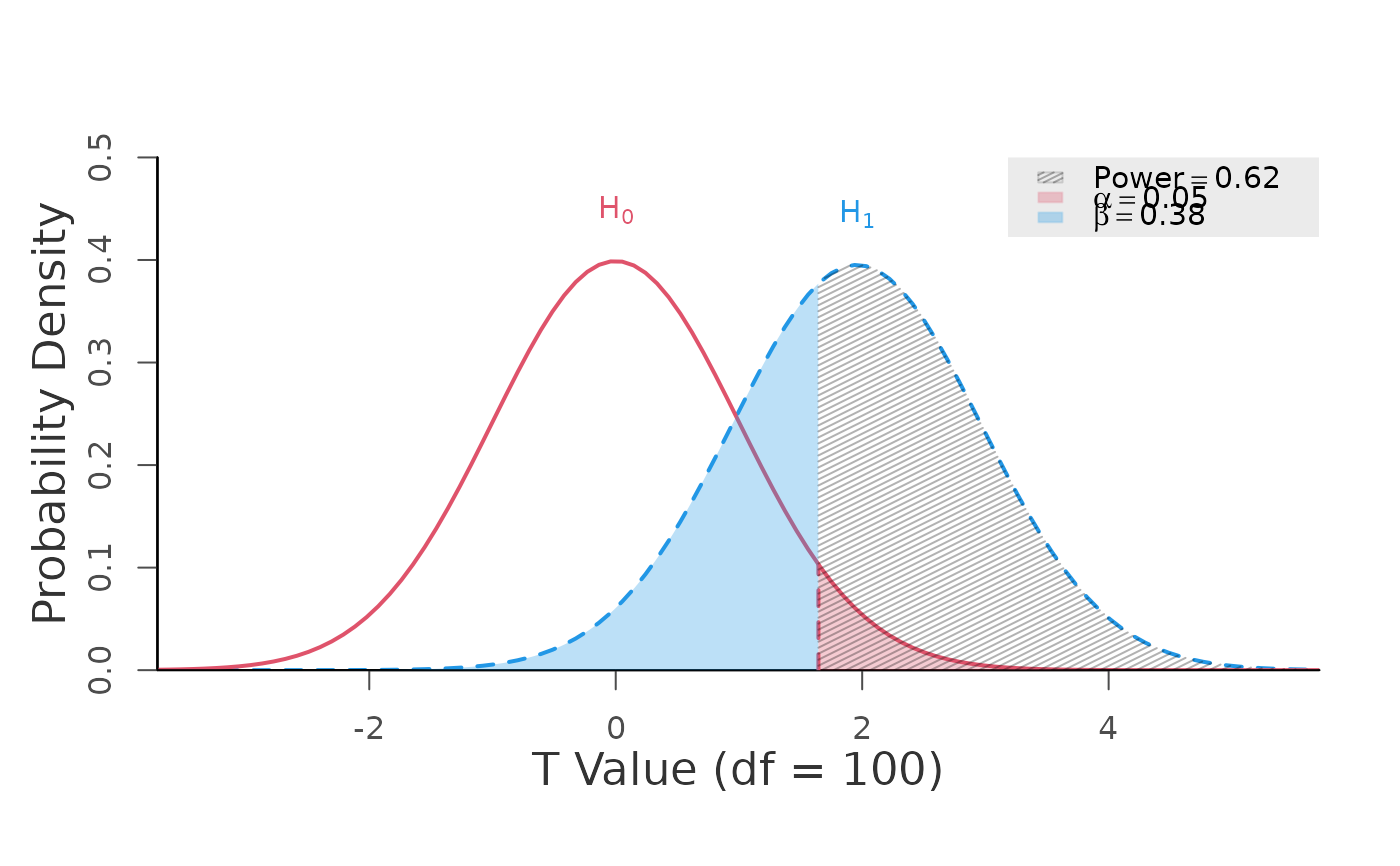
power.lp.test(ncp = 1.960, df = 100, alpha = 0.05, alternative = "one.sided")
 #> +--------------------------------------------------+
#> | POWER CALCULATION |
#> +--------------------------------------------------+
#>
#> Generic Lambda-Prime Distribution
#>
#> ----------------------------------------------------
#> Hypotheses
#> ----------------------------------------------------
#> H0 (Null) : lambda <= null.lambda
#> H1 (Alternative) : lambda > null.lambda
#>
#> ----------------------------------------------------
#> Results
#> ----------------------------------------------------
#> Target NCP (lambda) = 1.960 (vs. null.lambda = 0)
#> Degrees of Freedom = 100
#> Type 1 Error (alpha) = 0.050
#> Type 2 Error (beta) = 0.379
#> Statistical Power = 0.621 <<
#>
power.lp.test(power = 0.800, df = 100, alpha = 0.05, alternative = "one.sided")
#> +--------------------------------------------------+
#> | POWER CALCULATION |
#> +--------------------------------------------------+
#>
#> Generic Lambda-Prime Distribution
#>
#> ----------------------------------------------------
#> Hypotheses
#> ----------------------------------------------------
#> H0 (Null) : lambda <= null.lambda
#> H1 (Alternative) : lambda > null.lambda
#>
#> ----------------------------------------------------
#> Results
#> ----------------------------------------------------
#> Target NCP (lambda) = 1.960 (vs. null.lambda = 0)
#> Degrees of Freedom = 100
#> Type 1 Error (alpha) = 0.050
#> Type 2 Error (beta) = 0.379
#> Statistical Power = 0.621 <<
#>
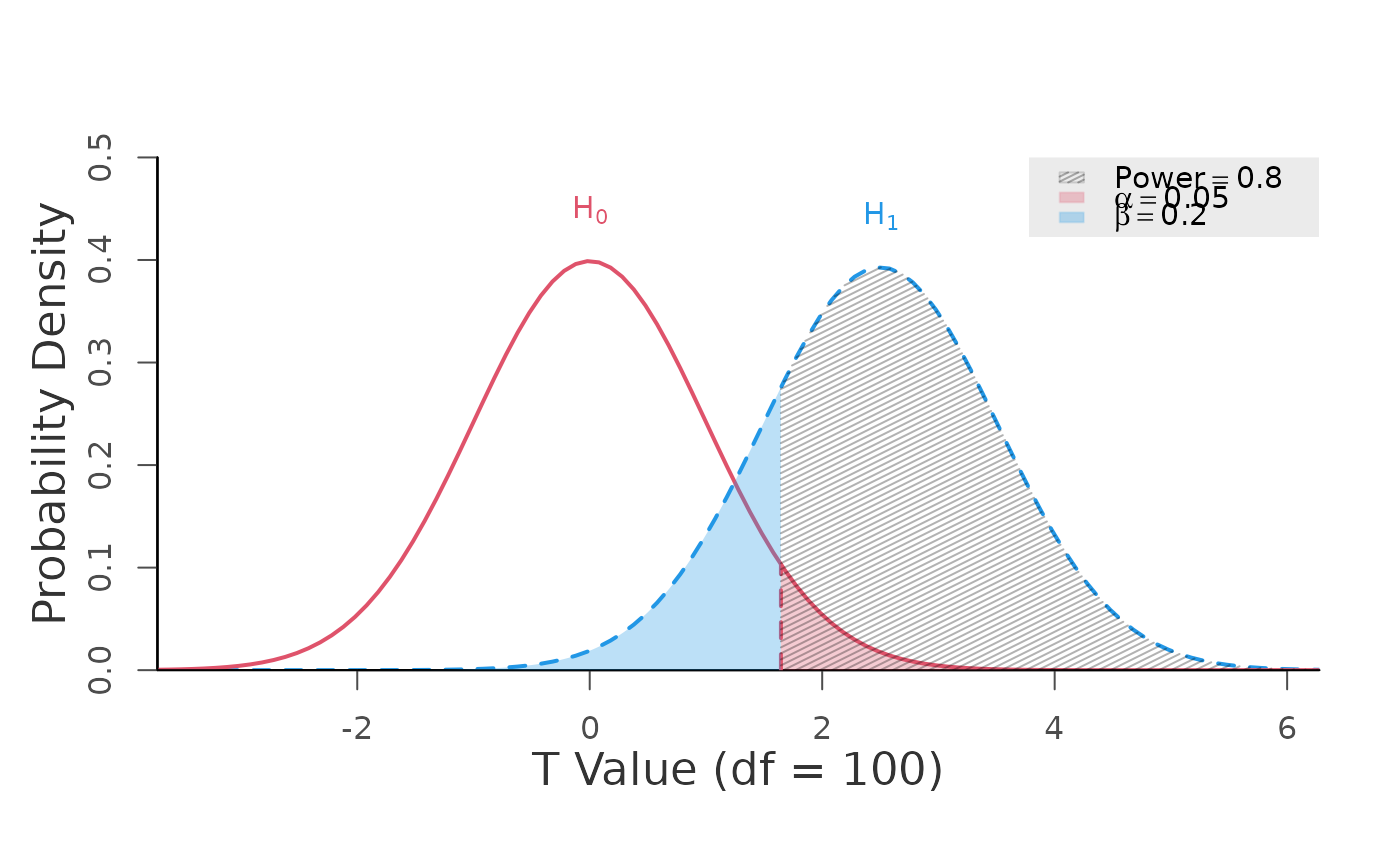
power.lp.test(power = 0.800, df = 100, alpha = 0.05, alternative = "one.sided")
 #> +--------------------------------------------------+
#> | MINIMUM DETECTABLE NCP CALCULATION |
#> +--------------------------------------------------+
#>
#> Generic Lambda-Prime Distribution
#>
#> ----------------------------------------------------
#> Hypotheses
#> ----------------------------------------------------
#> H0 (Null) : lambda <= null.lambda
#> H1 (Alternative) : lambda > null.lambda
#>
#> ----------------------------------------------------
#> Results
#> ----------------------------------------------------
#> Target NCP (lambda) = 2.506 (vs. null.lambda = 0) <<
#> Degrees of Freedom = 100
#> Type 1 Error (alpha) = 0.050
#> Type 2 Error (beta) = 0.200
#> Statistical Power = 0.800
#>
# the two examples below estimate the df's based upon the first example
# (revealing a power of 0.6207; df = 100.323) and the second example (revealing
# a ncp of 2.506; df = 99.12)
power.lp.test(ncp = 1.960, power = 0.6207, alpha = 0.05,
alternative = "one.sided", plot = FALSE)
#> +--------------------------------------------------+
#> | SAMPLE SIZE CALCULATION |
#> +--------------------------------------------------+
#>
#> Generic Lambda-Prime Distribution
#>
#> ----------------------------------------------------
#> Hypotheses
#> ----------------------------------------------------
#> H0 (Null) : lambda <= null.lambda
#> H1 (Alternative) : lambda > null.lambda
#>
#> ----------------------------------------------------
#> Results
#> ----------------------------------------------------
#> Target NCP (lambda) = 1.960 (vs. null.lambda = 0)
#> Degrees of Freedom = 100.323 <<
#> Type 1 Error (alpha) = 0.050
#> Type 2 Error (beta) = 0.379
#> Statistical Power = 0.621
#>
power.lp.test(ncp = 2.506, power = 0.8000, alpha = 0.05,
alternative = "one.sided", plot = FALSE)
#> +--------------------------------------------------+
#> | SAMPLE SIZE CALCULATION |
#> +--------------------------------------------------+
#>
#> Generic Lambda-Prime Distribution
#>
#> ----------------------------------------------------
#> Hypotheses
#> ----------------------------------------------------
#> H0 (Null) : lambda <= null.lambda
#> H1 (Alternative) : lambda > null.lambda
#>
#> ----------------------------------------------------
#> Results
#> ----------------------------------------------------
#> Target NCP (lambda) = 2.506 (vs. null.lambda = 0)
#> Degrees of Freedom = 99.12 <<
#> Type 1 Error (alpha) = 0.050
#> Type 2 Error (beta) = 0.200
#> Statistical Power = 0.800
#>
# equivalence
# power is defined as the probability of observing a test statistic greater
# than the upper critical value (for the lower bound) AND less than the
# lower critical value (for the upper bound)
power.lp.test(ncp = 0, null.ncp = c(-3, 3), df = 100, alpha = 0.05,
alternative = "two.one.sided", plot = FALSE)
#> +--------------------------------------------------+
#> | POWER CALCULATION |
#> +--------------------------------------------------+
#>
#> Generic Lambda-Prime Distribution
#>
#> ----------------------------------------------------
#> Hypotheses
#> ----------------------------------------------------
#> H0 (Null) : lambda <= min(null.lambda) or
#> lambda >= max(null.lambda)
#> H1 (Alternative) : lambda > min(null.lambda) and
#> lambda < max(null.lambda)
#>
#> ----------------------------------------------------
#> Results
#> ----------------------------------------------------
#> Target NCP (lambda) = 0 (vs. null.lambda = -3 and 3)
#> Degrees of Freedom = 100
#> Type 1 Error (alpha) = 0.050
#> Type 2 Error (beta) = 0.190
#> Statistical Power = 0.810 <<
#>
power.lp.test(power = 0.80, req.sign = "0", null.ncp = c(-3, 3),
df = 100, alpha = 0.05, alternative = "two.one.sided", plot = FALSE)
#> Warning: Target NCP ranges from -0.2157 to 0.2157 within the null bounds.
#> +--------------------------------------------------+
#> | MINIMUM DETECTABLE NCP CALCULATION |
#> +--------------------------------------------------+
#>
#> Generic Lambda-Prime Distribution
#>
#> ----------------------------------------------------
#> Hypotheses
#> ----------------------------------------------------
#> H0 (Null) : lambda <= min(null.lambda) or
#> lambda >= max(null.lambda)
#> H1 (Alternative) : lambda > min(null.lambda) and
#> lambda < max(null.lambda)
#>
#> ----------------------------------------------------
#> Results
#> ----------------------------------------------------
#> Target NCP (lambda) = 0 (vs. null.lambda = -3 and 3) <<
#> Degrees of Freedom = 100
#> Type 1 Error (alpha) = 0.050
#> Type 2 Error (beta) = 0.190
#> Statistical Power = 0.810
#>
# adjust the power based upon what is returned from the example above in
# order to get a valid estimate of the df's (100.321; power = 0.8 -> 58.911)
power.lp.test(ncp = 0, power = 0.8103, req.sign = "0", null.ncp = c(-3, 3),
alpha = 0.05, alternative = "two.one.sided", plot = FALSE)
#> +--------------------------------------------------+
#> | SAMPLE SIZE CALCULATION |
#> +--------------------------------------------------+
#>
#> Generic Lambda-Prime Distribution
#>
#> ----------------------------------------------------
#> Hypotheses
#> ----------------------------------------------------
#> H0 (Null) : lambda <= min(null.lambda) or
#> lambda >= max(null.lambda)
#> H1 (Alternative) : lambda > min(null.lambda) and
#> lambda < max(null.lambda)
#>
#> ----------------------------------------------------
#> Results
#> ----------------------------------------------------
#> Target NCP (lambda) = 0 (vs. null.lambda = -3 and 3)
#> Degrees of Freedom = 100.321 <<
#> Type 1 Error (alpha) = 0.050
#> Type 2 Error (beta) = 0.190
#> Statistical Power = 0.810
#>
# minimal effect testing
# power is defined as the probability of observing a test statistic greater
# than the upper critical value (for the upper bound) OR less than the lower
# critical value (for the lower bound).
power.lp.test(ncp = 2, null.ncp = c(-1, 1), df = 100, alpha = 0.05,
alternative = "two.one.sided", plot = FALSE)
#> +--------------------------------------------------+
#> | POWER CALCULATION |
#> +--------------------------------------------------+
#>
#> Generic Lambda-Prime Distribution
#>
#> ----------------------------------------------------
#> Hypotheses
#> ----------------------------------------------------
#> H0 (Null) : lambda >= min(null.lambda) and
#> lambda <= max(null.lambda)
#> H1 (Alternative) : lambda < min(null.lambda) or
#> lambda > max(null.lambda)
#>
#> ----------------------------------------------------
#> Results
#> ----------------------------------------------------
#> Target NCP (lambda) = 2 (vs. null.lambda = -1 and 1)
#> Degrees of Freedom = 100
#> Type 1 Error (alpha) = 0.050
#> Type 2 Error (beta) = 0.831
#> Statistical Power = 0.169 <<
#>
power.lp.test(power = 0.80, req.sign = "+", null.ncp = c(-1, 1),
df = 100, alpha = 0.05, alternative = "two.one.sided")
#> +--------------------------------------------------+
#> | MINIMUM DETECTABLE NCP CALCULATION |
#> +--------------------------------------------------+
#>
#> Generic Lambda-Prime Distribution
#>
#> ----------------------------------------------------
#> Hypotheses
#> ----------------------------------------------------
#> H0 (Null) : lambda <= null.lambda
#> H1 (Alternative) : lambda > null.lambda
#>
#> ----------------------------------------------------
#> Results
#> ----------------------------------------------------
#> Target NCP (lambda) = 2.506 (vs. null.lambda = 0) <<
#> Degrees of Freedom = 100
#> Type 1 Error (alpha) = 0.050
#> Type 2 Error (beta) = 0.200
#> Statistical Power = 0.800
#>
# the two examples below estimate the df's based upon the first example
# (revealing a power of 0.6207; df = 100.323) and the second example (revealing
# a ncp of 2.506; df = 99.12)
power.lp.test(ncp = 1.960, power = 0.6207, alpha = 0.05,
alternative = "one.sided", plot = FALSE)
#> +--------------------------------------------------+
#> | SAMPLE SIZE CALCULATION |
#> +--------------------------------------------------+
#>
#> Generic Lambda-Prime Distribution
#>
#> ----------------------------------------------------
#> Hypotheses
#> ----------------------------------------------------
#> H0 (Null) : lambda <= null.lambda
#> H1 (Alternative) : lambda > null.lambda
#>
#> ----------------------------------------------------
#> Results
#> ----------------------------------------------------
#> Target NCP (lambda) = 1.960 (vs. null.lambda = 0)
#> Degrees of Freedom = 100.323 <<
#> Type 1 Error (alpha) = 0.050
#> Type 2 Error (beta) = 0.379
#> Statistical Power = 0.621
#>
power.lp.test(ncp = 2.506, power = 0.8000, alpha = 0.05,
alternative = "one.sided", plot = FALSE)
#> +--------------------------------------------------+
#> | SAMPLE SIZE CALCULATION |
#> +--------------------------------------------------+
#>
#> Generic Lambda-Prime Distribution
#>
#> ----------------------------------------------------
#> Hypotheses
#> ----------------------------------------------------
#> H0 (Null) : lambda <= null.lambda
#> H1 (Alternative) : lambda > null.lambda
#>
#> ----------------------------------------------------
#> Results
#> ----------------------------------------------------
#> Target NCP (lambda) = 2.506 (vs. null.lambda = 0)
#> Degrees of Freedom = 99.12 <<
#> Type 1 Error (alpha) = 0.050
#> Type 2 Error (beta) = 0.200
#> Statistical Power = 0.800
#>
# equivalence
# power is defined as the probability of observing a test statistic greater
# than the upper critical value (for the lower bound) AND less than the
# lower critical value (for the upper bound)
power.lp.test(ncp = 0, null.ncp = c(-3, 3), df = 100, alpha = 0.05,
alternative = "two.one.sided", plot = FALSE)
#> +--------------------------------------------------+
#> | POWER CALCULATION |
#> +--------------------------------------------------+
#>
#> Generic Lambda-Prime Distribution
#>
#> ----------------------------------------------------
#> Hypotheses
#> ----------------------------------------------------
#> H0 (Null) : lambda <= min(null.lambda) or
#> lambda >= max(null.lambda)
#> H1 (Alternative) : lambda > min(null.lambda) and
#> lambda < max(null.lambda)
#>
#> ----------------------------------------------------
#> Results
#> ----------------------------------------------------
#> Target NCP (lambda) = 0 (vs. null.lambda = -3 and 3)
#> Degrees of Freedom = 100
#> Type 1 Error (alpha) = 0.050
#> Type 2 Error (beta) = 0.190
#> Statistical Power = 0.810 <<
#>
power.lp.test(power = 0.80, req.sign = "0", null.ncp = c(-3, 3),
df = 100, alpha = 0.05, alternative = "two.one.sided", plot = FALSE)
#> Warning: Target NCP ranges from -0.2157 to 0.2157 within the null bounds.
#> +--------------------------------------------------+
#> | MINIMUM DETECTABLE NCP CALCULATION |
#> +--------------------------------------------------+
#>
#> Generic Lambda-Prime Distribution
#>
#> ----------------------------------------------------
#> Hypotheses
#> ----------------------------------------------------
#> H0 (Null) : lambda <= min(null.lambda) or
#> lambda >= max(null.lambda)
#> H1 (Alternative) : lambda > min(null.lambda) and
#> lambda < max(null.lambda)
#>
#> ----------------------------------------------------
#> Results
#> ----------------------------------------------------
#> Target NCP (lambda) = 0 (vs. null.lambda = -3 and 3) <<
#> Degrees of Freedom = 100
#> Type 1 Error (alpha) = 0.050
#> Type 2 Error (beta) = 0.190
#> Statistical Power = 0.810
#>
# adjust the power based upon what is returned from the example above in
# order to get a valid estimate of the df's (100.321; power = 0.8 -> 58.911)
power.lp.test(ncp = 0, power = 0.8103, req.sign = "0", null.ncp = c(-3, 3),
alpha = 0.05, alternative = "two.one.sided", plot = FALSE)
#> +--------------------------------------------------+
#> | SAMPLE SIZE CALCULATION |
#> +--------------------------------------------------+
#>
#> Generic Lambda-Prime Distribution
#>
#> ----------------------------------------------------
#> Hypotheses
#> ----------------------------------------------------
#> H0 (Null) : lambda <= min(null.lambda) or
#> lambda >= max(null.lambda)
#> H1 (Alternative) : lambda > min(null.lambda) and
#> lambda < max(null.lambda)
#>
#> ----------------------------------------------------
#> Results
#> ----------------------------------------------------
#> Target NCP (lambda) = 0 (vs. null.lambda = -3 and 3)
#> Degrees of Freedom = 100.321 <<
#> Type 1 Error (alpha) = 0.050
#> Type 2 Error (beta) = 0.190
#> Statistical Power = 0.810
#>
# minimal effect testing
# power is defined as the probability of observing a test statistic greater
# than the upper critical value (for the upper bound) OR less than the lower
# critical value (for the lower bound).
power.lp.test(ncp = 2, null.ncp = c(-1, 1), df = 100, alpha = 0.05,
alternative = "two.one.sided", plot = FALSE)
#> +--------------------------------------------------+
#> | POWER CALCULATION |
#> +--------------------------------------------------+
#>
#> Generic Lambda-Prime Distribution
#>
#> ----------------------------------------------------
#> Hypotheses
#> ----------------------------------------------------
#> H0 (Null) : lambda >= min(null.lambda) and
#> lambda <= max(null.lambda)
#> H1 (Alternative) : lambda < min(null.lambda) or
#> lambda > max(null.lambda)
#>
#> ----------------------------------------------------
#> Results
#> ----------------------------------------------------
#> Target NCP (lambda) = 2 (vs. null.lambda = -1 and 1)
#> Degrees of Freedom = 100
#> Type 1 Error (alpha) = 0.050
#> Type 2 Error (beta) = 0.831
#> Statistical Power = 0.169 <<
#>
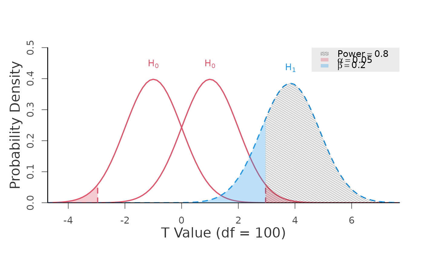
power.lp.test(power = 0.80, req.sign = "+", null.ncp = c(-1, 1),
df = 100, alpha = 0.05, alternative = "two.one.sided")
 #> +--------------------------------------------------+
#> | MINIMUM DETECTABLE NCP CALCULATION |
#> +--------------------------------------------------+
#>
#> Generic Lambda-Prime Distribution
#>
#> ----------------------------------------------------
#> Hypotheses
#> ----------------------------------------------------
#> H0 (Null) : lambda >= min(null.lambda) and
#> lambda <= max(null.lambda)
#> H1 (Alternative) : lambda < min(null.lambda) or
#> lambda > max(null.lambda)
#>
#> ----------------------------------------------------
#> Results
#> ----------------------------------------------------
#> Target NCP (lambda) = 3.844 (vs. null.lambda = -1 and 1) <<
#> Degrees of Freedom = 100
#> Type 1 Error (alpha) = 0.050
#> Type 2 Error (beta) = 0.200
#> Statistical Power = 0.800
#>
# the first example (ncp = 2) reveals insufficient power (0.169), hence
# use the ncp returned from the example above for estimating the df's
power.lp.test(ncp = 3.844, power = 0.8, req.sign = "+", null.ncp = c(-3, 3),
alpha = 0.05, alternative = "two.one.sided", plot = FALSE)
#> +--------------------------------------------------+
#> | SAMPLE SIZE CALCULATION |
#> +--------------------------------------------------+
#>
#> Generic Lambda-Prime Distribution
#>
#> ----------------------------------------------------
#> Hypotheses
#> ----------------------------------------------------
#> H0 (Null) : lambda >= min(null.lambda) and
#> lambda <= max(null.lambda)
#> H1 (Alternative) : lambda < min(null.lambda) or
#> lambda > max(null.lambda)
#>
#> ----------------------------------------------------
#> Results
#> ----------------------------------------------------
#> Target NCP (lambda) = 3.844 (vs. null.lambda = -3 and 3)
#> Degrees of Freedom = 9999844144.626 <<
#> Type 1 Error (alpha) = 0.050
#> Type 2 Error (beta) = 0.868
#> Statistical Power = 0.132
#>
#> +--------------------------------------------------+
#> | MINIMUM DETECTABLE NCP CALCULATION |
#> +--------------------------------------------------+
#>
#> Generic Lambda-Prime Distribution
#>
#> ----------------------------------------------------
#> Hypotheses
#> ----------------------------------------------------
#> H0 (Null) : lambda >= min(null.lambda) and
#> lambda <= max(null.lambda)
#> H1 (Alternative) : lambda < min(null.lambda) or
#> lambda > max(null.lambda)
#>
#> ----------------------------------------------------
#> Results
#> ----------------------------------------------------
#> Target NCP (lambda) = 3.844 (vs. null.lambda = -1 and 1) <<
#> Degrees of Freedom = 100
#> Type 1 Error (alpha) = 0.050
#> Type 2 Error (beta) = 0.200
#> Statistical Power = 0.800
#>
# the first example (ncp = 2) reveals insufficient power (0.169), hence
# use the ncp returned from the example above for estimating the df's
power.lp.test(ncp = 3.844, power = 0.8, req.sign = "+", null.ncp = c(-3, 3),
alpha = 0.05, alternative = "two.one.sided", plot = FALSE)
#> +--------------------------------------------------+
#> | SAMPLE SIZE CALCULATION |
#> +--------------------------------------------------+
#>
#> Generic Lambda-Prime Distribution
#>
#> ----------------------------------------------------
#> Hypotheses
#> ----------------------------------------------------
#> H0 (Null) : lambda >= min(null.lambda) and
#> lambda <= max(null.lambda)
#> H1 (Alternative) : lambda < min(null.lambda) or
#> lambda > max(null.lambda)
#>
#> ----------------------------------------------------
#> Results
#> ----------------------------------------------------
#> Target NCP (lambda) = 3.844 (vs. null.lambda = -3 and 3)
#> Degrees of Freedom = 9999844144.626 <<
#> Type 1 Error (alpha) = 0.050
#> Type 2 Error (beta) = 0.868
#> Statistical Power = 0.132
#>