Cate-Nelson models for bivariate data with a fixed critical Y value

Produces critical-x values for bivariate data according to a Cate-Nelson analysis for a given critical Y value.

Usage

cateNelsonFixedY(
  x,
  y,
  cly = 0.95,
  plotit = TRUE,
  hollow = TRUE,
  xlab = "X",
  ylab = "Y",
  trend = "positive",
  clx = 1,
  outlength = 20,
  sortstat = "error"
)

Arguments

x: A vector of values for the x variable.
y: A vector of values for the y variable.
cly: = Critical Y value.
plotit: If TRUE, produces plots of the output.
hollow: If TRUE, uses hollow circles on the plot to indicate data not fitting the model.
xlab: The label for the x-axis.
ylab: The label for the y-axis.
trend: "postive" if the trend of y vs. x is generally positive. "negative" if negative.
clx: Indicates which of the listed critical x values should be chosen as the critical x value for the plot.
outlength: Indicates the number of potential critical x values to display in the output.
sortstat: The statistic to sort by. Any of "error" (the default), "phi", "fisher", or "pearson".

Value

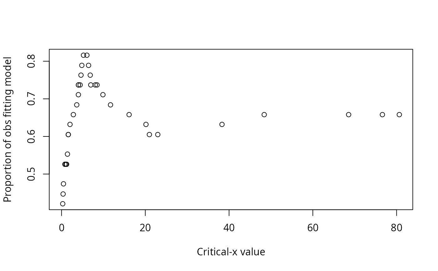
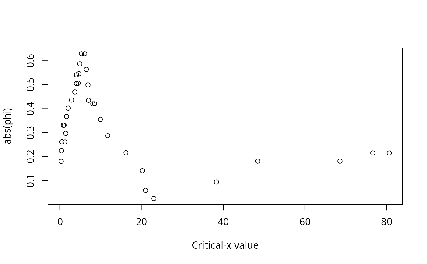
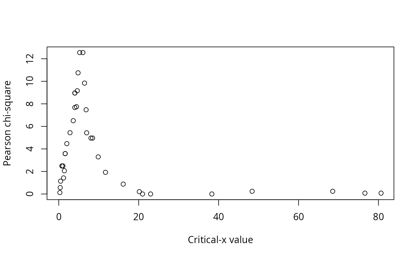
A data frame of statistics from the analysis: critical level for x, critical value for y, the number of observations in each of the quadrants (I, II, III, IV), the number of observations that conform with the model, the number of observations that do not conform to the model, the proportion of observations that conform with the model, the proportion of observations that do not conform to the model, a p-value for the Fisher exact test for the data divided into the groups indicated by the model, phi for the data divided into the groups indicated by the model, and Pearson's chi-square for the data divided into the groups indicated by the model.

Details

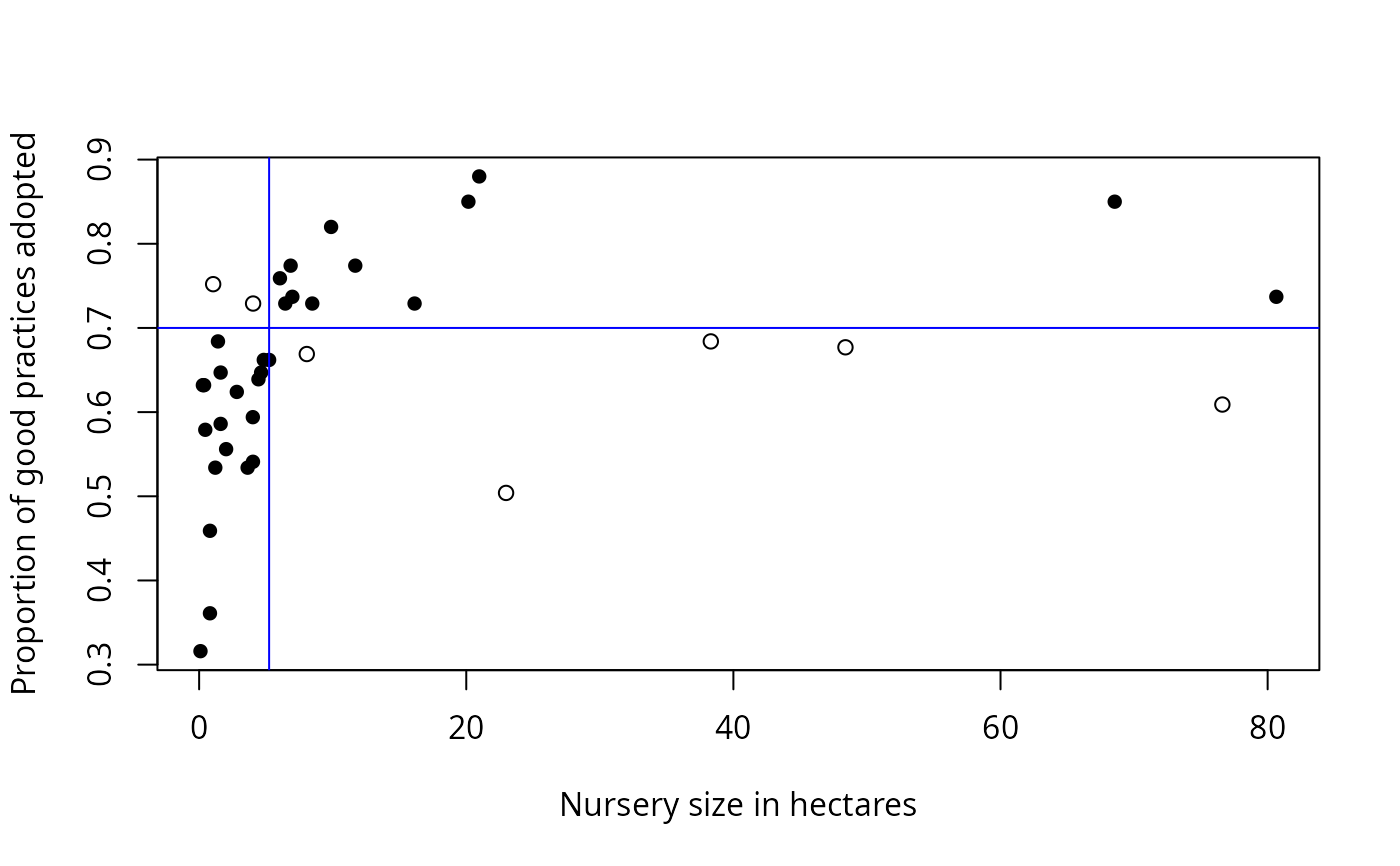
Cate-Nelson analysis divides bivariate data into two groups. For data with a positive trend, one group has a large x value associated with a large y value, and the other group has a small x value associated with a small y value. For a negative trend, a small x is associated with a large y, and so on.

The analysis is useful for bivariate data which don't conform well to linear, curvilinear, or plateau models.

References

https://rcompanion.org/rcompanion/h_02.html

Author

Salvatore Mangiafico, mangiafico@njaes.rutgers.edu

Examples

data(Nurseries)
cateNelsonFixedY(x          = Nurseries$Size,
                 y          = Nurseries$Proportion,
                 cly        = 0.70,
                 plotit     = TRUE,
                 hollow     = TRUE,
                 xlab       = "Nursery size in hectares",
                 ylab       = "Proportion of good practices adopted",
                 trend      = "positive",
                 clx        = 1,
                 outlength  = 15)




#>    Critx Crity Q1 Q2 Q3 Q4 Model Error  N   pQ1   pQ2   pQ3   pQ4 pModel pError
#> 1   5.24   0.7  2 12  5 19    31     7 38 0.053 0.316 0.132 0.500  0.816  0.184
#> 2   6.05   0.7  2 12  5 19    31     7 38 0.053 0.316 0.132 0.500  0.816  0.184
#> 3   4.84   0.7  2 12  6 18    30     8 38 0.053 0.316 0.158 0.474  0.789  0.211
#> 4   6.45   0.7  3 11  5 19    30     8 38 0.079 0.289 0.132 0.500  0.789  0.211
#> 5   4.64   0.7  2 12  7 17    29     9 38 0.053 0.316 0.184 0.447  0.763  0.237
#> 6   6.85   0.7  4 10  5 19    29     9 38 0.105 0.263 0.132 0.500  0.763  0.237
#> 7   4.03   0.7  1 13  9 15    28    10 38 0.026 0.342 0.237 0.395  0.737  0.263
#> 8   4.04   0.7  1 13  9 15    28    10 38 0.026 0.342 0.237 0.395  0.737  0.263
#> 9   4.44   0.7  2 12  8 16    28    10 38 0.053 0.316 0.211 0.421  0.737  0.263
#> 10  6.98   0.7  5  9  5 19    28    10 38 0.132 0.237 0.132 0.500  0.737  0.263
#> 11  8.06   0.7  6  8  4 20    28    10 38 0.158 0.211 0.105 0.526  0.737  0.263
#> 12  8.47   0.7  6  8  4 20    28    10 38 0.158 0.211 0.105 0.526  0.737  0.263
#> 13  4.02   0.7  1 13 10 14    27    11 38 0.026 0.342 0.263 0.368  0.711  0.289
#> 14  9.88   0.7  7  7  4 20    27    11 38 0.184 0.184 0.105 0.526  0.711  0.289
#> 15  3.63   0.7  1 13 11 13    26    12 38 0.026 0.342 0.289 0.342  0.684  0.316
#>     Fisher.p Pearson.chisq Pearson.p    phi
#> 1  0.0001517        12.550 0.0003972 -0.629
#> 2  0.0001517        12.550 0.0003972 -0.629
#> 3  0.0005311        10.750 0.0010420 -0.587
#> 4  0.0007735         9.840 0.0017080 -0.564
#> 5  0.0018910         9.161 0.0024730 -0.546
#> 6  0.0048710         7.474 0.0062580 -0.499
#> 7  0.0015970         8.961 0.0027590 -0.541
#> 8  0.0015970         8.961 0.0027590 -0.541
#> 9  0.0025240         7.744 0.0053900 -0.506
#> 10 0.0138000         5.429 0.0198100 -0.435
#> 11 0.0143900         4.962 0.0259100 -0.420
#> 12 0.0143900         4.962 0.0259100 -0.420
#> 13 0.0021210         7.674 0.0056030 -0.505
#> 14 0.0607300         3.293 0.0695600 -0.355
#> 15 0.0049960         6.503 0.0107700 -0.470