3-D Plots Showing Effects of Two Continuous Predictors in a Regression Model Fit

Uses lattice graphics and the output from Predict to plot image, contour, or perspective plots showing the simultaneous effects of two continuous predictor variables. Unless formula is provided, the \(x\)-axis is constructed from the first variable listed in the call to Predict and the \(y\)-axis variable comes from the second.

The perimeter function is used to generate the boundary of data to plot when a 3-d plot is made. It finds the area where there are sufficient data to generate believable interaction fits.

bplot(x, formula, lfun=lattice::levelplot, xlab, ylab, zlab,
      adj.subtitle=!info$ref.zero, cex.adj=.75, cex.lab=1,
      perim, showperim=FALSE,
      zlim=range(yhat, na.rm=TRUE), scales=list(arrows=FALSE),
      xlabrot, ylabrot, zlabrot=90, ...)

perimeter(x, y, xinc=diff(range(x))/10, n=10, lowess.=TRUE)

Arguments

x: for bplot, an object created by Predict for which two or more numeric predictors varied. For perim is the first variable of a pair of predictors forming a 3-d plot.
formula: a formula of the form f(yhat) ~ x*y optionally followed by |a*b*c which are 1-3 paneling variables that were specified to Predict. f can represent any R function of a vector that produces a vector. If the left hand side of the formula is omitted, yhat will be inserted. If formula is omitted, it will be inferred from the first two variables that varied in the call to Predict.
lfun: a high-level lattice plotting function that takes formulas of the form z ~ x*y. The default is an image plot (levelplot). Other common choices are wireframe for perspective plot or contourplot for a contour plot.
xlab: Character string label for \(x\)-axis. Default is given by Predict.
ylab: Character string abel for \(y\)-axis
zlab: Character string \(z\)-axis label for perspective (wireframe) plots. Default comes from Predict. zlab will often be specified if fun was specified to Predict.
adj.subtitle: Set to FALSE to suppress subtitling the graph with the list of settings of non-graphed adjustment values. Default is TRUE if there are non-plotted adjustment variables and ref.zero was not used.
cex.adj: cex parameter for size of adjustment settings in subtitles. Default is 0.75
cex.lab: cex parameter for axis labels. Default is 1.
perim: names a matrix created by perimeter when used for 3-d plots of two continuous predictors. When the combination of variables is outside the range in perim, that section of the plot is suppressed. If perim is omitted, 3-d plotting will use the marginal distributions of the two predictors to determine the plotting region, when the grid is not specified explicitly in variables. When instead a series of curves is being plotted, perim specifies a function having two arguments. The first is the vector of values of the first variable that is about to be plotted on the \(x\)-axis. The second argument is the single value of the variable representing different curves, for the current curve being plotted. The function's returned value must be a logical vector whose length is the same as that of the first argument, with values TRUE if the corresponding point should be plotted for the current curve, FALSE otherwise. See one of the latter examples.
showperim: set to TRUE if perim is specified and you want to show the actual perimeter used.
zlim: Controls the range for plotting in the \(z\)-axis if there is one. Computed by default.
scales: see wireframe
xlabrot: rotation angle for the x-axis. Default is 30 for wireframe and 0 otherwise.
ylabrot: rotation angle for the y-axis. Default is -40 for wireframe, 90 for contourplot or levelplot, and 0 otherwise.
zlabrot: rotation angle for z-axis rotation for wireframe plots
...: other arguments to pass to the lattice function
y: second variable of the pair for perim. If omitted, x is assumed to be a list with both x and y components.
xinc: increment in x over which to examine the density of y in perimeter
n: within intervals of x for perimeter, takes the informative range of y to be the \(n\)th smallest to the \(n\)th largest values of y. If there aren't at least 2\(n\) y values in the x interval, no y ranges are used for that interval.
lowess.: set to FALSE to not have lowess smooth the data perimeters

Value

perimeter returns a matrix of class perimeter. This outline can be conveniently plotted by lines.perimeter.

Details

perimeter is a kind of generalization of datadist for 2 continuous variables. First, the n smallest and largest x values are determined. These form the lowest and highest possible xs to display. Then x is grouped into intervals bounded by these two numbers, with the interval widths defined by xinc. Within each interval, y is sorted and the \(n\)th smallest and largest y are taken as the interval containing sufficient data density to plot interaction surfaces. The interval is ignored when there are insufficient y values. When the data are being readied for persp, bplot uses the approx function to do linear interpolation of the y-boundaries as a function of the x values actually used in forming the grid (the values of the first variable specified to Predict). To make the perimeter smooth, specify lowess.=TRUE to perimeter.

Author

Frank Harrell
Department of Biostatistics, Vanderbilt University
fh@fharrell.com

Examples

n <- 1000    # define sample size
set.seed(17) # so can reproduce the results
age            <- rnorm(n, 50, 10)
blood.pressure <- rnorm(n, 120, 15)
cholesterol    <- rnorm(n, 200, 25)
sex            <- factor(sample(c('female','male'), n,TRUE))
label(age)            <- 'Age'      # label is in Hmisc
label(cholesterol)    <- 'Total Cholesterol'
label(blood.pressure) <- 'Systolic Blood Pressure'
label(sex)            <- 'Sex'
units(cholesterol)    <- 'mg/dl'   # uses units.default in Hmisc
units(blood.pressure) <- 'mmHg'

# Specify population model for log odds that Y=1
L <- .4*(sex=='male') + .045*(age-50) +
  (log(cholesterol - 10)-5.2)*(-2*(sex=='female') + 2*(sex=='male'))
# Simulate binary y to have Prob(y=1) = 1/[1+exp(-L)]
y <- ifelse(runif(n) < plogis(L), 1, 0)

ddist <- datadist(age, blood.pressure, cholesterol, sex)
options(datadist='ddist')

fit <- lrm(y ~ blood.pressure + sex * (age + rcs(cholesterol,4)),
               x=TRUE, y=TRUE)
#> Error in Design(data, formula = formula): dataset ddist not found for options(datadist=)
p <- Predict(fit, age, cholesterol, sex, np=50) # vary sex last
#> Error: object 'fit' not found
require(lattice)
bplot(p)                 # image plot for age, cholesterol with color
#> Error: object 'p' not found
                         # coming from yhat; use default ranges for
                         # both continuous predictors; two panels (for sex)
bplot(p, lfun=wireframe) # same as bplot(p,,wireframe)
#> Error: object 'p' not found
# View from different angle, change y label orientation accordingly
# Default is z=40, x=-60
bplot(p,, wireframe, screen=list(z=40, x=-75), ylabrot=-25)
#> Error: object 'p' not found
bplot(p,, contourplot)   # contour plot
#> Error: object 'p' not found
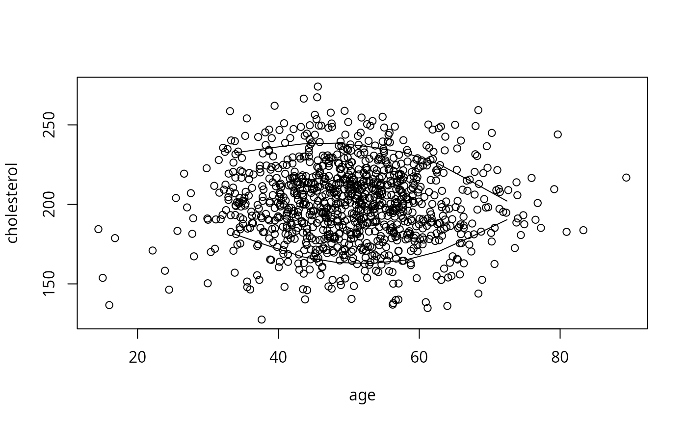
bounds  <- perimeter(age, cholesterol, lowess=TRUE)
plot(age, cholesterol)     # show bivariate data density and perimeter
lines(bounds[,c('x','ymin')]); lines(bounds[,c('x','ymax')])

p <- Predict(fit, age, cholesterol)  # use only one sex
#> Error: object 'fit' not found
bplot(p, perim=bounds)   # draws image() plot
#> Error: object 'p' not found
                         # don't show estimates where data are sparse
                         # doesn't make sense here since vars don't interact
bplot(p, plogis(yhat) ~ age*cholesterol) # Probability scale
#> Error: object 'p' not found
options(datadist=NULL)